
Dickens wrote fourteen and a half novels. I will start from analyzing five of them - “A Tale of Two Cities”, “Great Expectations”, “A Christmas Carol in Prose; Being a Ghost Story of Christmas”, “Oliver Twist” and “Hard Times”.
Project Gutenberg offers over 53,000 free books. I will download Dickens’ novels in UTF-8 encoded texts from there using gutenbergr package developed by David Robinson. Besides, I will be using the following packages for this project.
library(dplyr)
library(tm.plugin.webmining)
library(purrr)
library(tidytext)
library(gutenbergr)
library(ggplot2)
dickens <- gutenberg_download(c(98, 1400, 46, 730, 786))Download Dickens’ five novels by Project Gutenberg ID numbers.
tidy_dickens <- dickens %>%
  unnest_tokens(word, text) %>%
  anti_join(stop_words)
The unnest_tokens package is used to split each row so that there is one token (word) in each row of the new data frame (tidy_dickens). Then remove stop words with an anti_join function.
tidy_dickens %>%
  count(word, sort = TRUE)
### A tibble: 19,634 × 2
## word n
## <chr> <int>
##1 time 1218
##2 hand 918
##3 night 835
##4 looked 814
##5 head 813
##6 oliver 766
##7 dear 751
##8 joe 718
##9 miss 702
##10 sir 697
### ... with 19,624 more rowsAfter removing the stop words, here is a list of words starts from the most frequent.
tidy_dickens %>%
  count(word, sort = TRUE) %>%
  filter(n > 600) %>%
  mutate(word = reorder(word, n)) %>%
  ggplot(aes(word, n)) +
  geom_col() +
  xlab(NULL) +
  coord_flip() + ggtitle("The Most Common Words in Charles Dickens' Novels")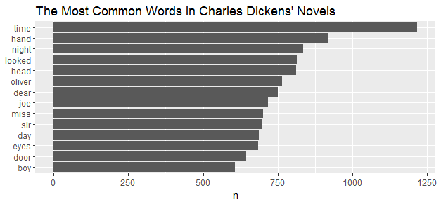
Sentiment in Dickens’ Five Novels
tidytext package contains several sentiment lexicons, I am using “bing” for the following tasks.
bing_word_counts <- tidy_dickens %>%
  inner_join(get_sentiments("bing")) %>%
  count(word, sentiment, sort = TRUE) %>%
  ungroup()
bing_word_counts
### A tibble: 3,145 × 3
## word sentiment n
## <chr> <chr> <int>
##1 miss negative 702
##2 poor negative 350
##3 dark negative 299
##4 hard negative 223
##5 dead negative 218
##6 strong positive 203
##7 love positive 202
##8 fell negative 198
##9 death negative 194
##10 cold negative 192
### ... with 3,135 more rowsHere I got the sentiment categories of Dickens’ words.
bing_word_counts %>%
  group_by(sentiment) %>%
  top_n(10) %>%
  ungroup() %>%
  mutate(word = reorder(word, n)) %>%
  ggplot(aes(word, n, fill = sentiment)) +
  geom_col(show.legend = FALSE) +
  facet_wrap(~sentiment, scales = "free_y") +
  labs(y = "Words Contribute to sentiment",
       x = NULL) +
  coord_flip()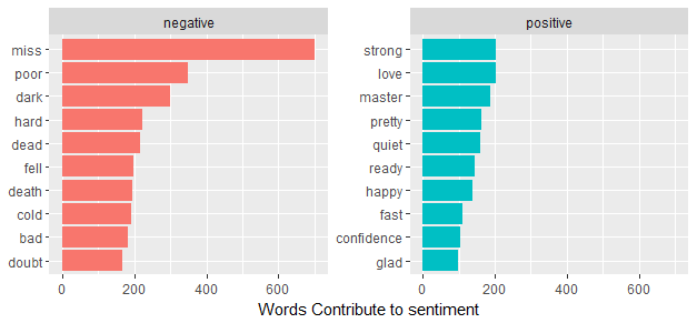
The word “miss” is the most frequent negative word here, but it is used to describe unmarried women in Dickens’ works. In particualr, Miss Havisham is a significant character in the Charles Dickens novel “Great Expectations”. Dickens describes her as looking like “the witch of the place”. In this case, probably “miss”” should be a negative word.
Oh poor Pip!
library(wordcloud)
tidy_dickens %>%
  anti_join(stop_words) %>%
  count(word) %>%
  with(wordcloud(word, n, max.words = 100))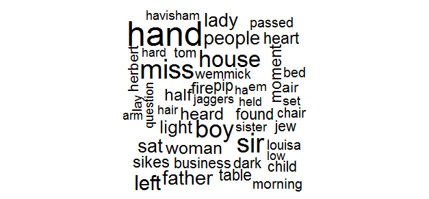
Word cloud is a good idea to identify trends and patterns that would otherwise be unclear or difficult to see in a tabular format.
library(reshape2)
tidy_dickens %>%
  inner_join(get_sentiments("bing")) %>%
  count(word, sentiment, sort = TRUE) %>%
  acast(word ~ sentiment, value.var = "n", fill = 0) %>%
  comparison.cloud(colors = c("#F8766D", "#00BFC4"),
                   max.words = 100)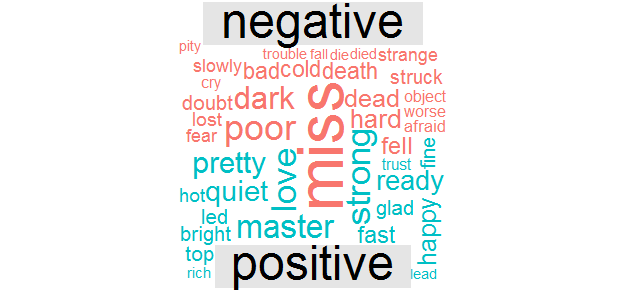
And compare most frequent positive and negative words in word cloud.
Relationships between words
dickens_bigrams <- dickens %>%
  unnest_tokens(bigram, text, token = "ngrams", n = 2)
dickens_bigrams
### A tibble: 616,994 × 2
## gutenberg_id bigram
## <int> <chr>
##1 46 a christmas
##2 46 christmas carol
##3 46 carol in
##4 46 in prose
##5 46 prose being
##6 46 being a
##7 46 a ghost
##8 46 ghost story
##9 46 story of
##10 46 of christmas
### ... with 616,984 more rowsEach token now represents a bigram (two words paired). if one of the words in the bigram is a stop word, this word will be removed. After filtering out stop words, what are the most frequent bigrams?
library(tidyr)
bigrams_separated <- dickens_bigrams %>%
  separate(bigram, c("word1", "word2"), sep = " ")
bigrams_filtered <- bigrams_separated %>%
  filter(!word1 %in% stop_words$word) %>%
  filter(!word2 %in% stop_words$word)
bigram_counts <- bigrams_filtered %>%
  count(word1, word2, sort = TRUE)
bigram_counts
##Source: local data frame [41,584 x 3]
##Groups: word1 [10,206]
## word1 word2 n
## <chr> <chr> <int>
##1 miss havisham 236
##2 miss pross 144
##3 madame defarge 113
##4 dear boy 77
##5 ha ha 77
##6 doctor manette 75
##7 miss havisham's 74
##8 oliver twist 55
##9 sir replied 54
##10 wine shop 52
### ... with 41,574 more rowsNames are the most common paired words in Dickens’ novels.
bigrams_united <- bigrams_filtered %>%
  unite(bigram, word1, word2, sep = " ")
bigrams_united
### A tibble: 51,379 × 2
## gutenberg_id bigram
##* <int> <chr>
##1 46 christmas carol
##2 46 ghost story
##3 46 charles dickens
##4 46 dickens preface
##5 46 houses pleasantly
##6 46 faithful friend
##7 46 december 1843
##8 46 1843 contents
##9 46 contents stave
##10 46 marley's ghost
### ... with 51,369 more rowsBefore visualizing it, I have to make these bigrams back to be united.
bigram_tf_idf <- bigrams_united %>%
  count(bigram)
bigram_tf_idf <- bigram_tf_idf %>% filter(n>30)
ggplot(aes(x = reorder(bigram, n), y=n), data=bigram_tf_idf) + geom_bar(stat = 'identity') + ggtitle("The Most Common Bigrams in Dickens' novels") + coord_flip()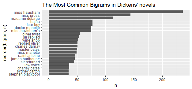
Yes, the most frequent bigrams in Dickens’ works are names. I also notice some pairings of a common verb such as “wine shop” from “A Tale of Two Cities” and “oliver twist”.
At last, visualizing a network of bigrams of Dickens’ five novels.
library(igraph)
bigram_graph <- bigram_counts %>%
  filter(n > 20) %>%
  graph_from_data_frame()
bigram_graph
##IGRAPH DN-- 61 37 --
##+ attr: name (v/c), n (e/n)
##+ edges (vertex names):
## [1] miss ->havisham miss ->pross madame ->defarge
## [4] dear ->boy ha ->ha doctor ->manette
## [7] miss ->havisham's oliver ->twist sir ->replied
##[10] wine ->shop charles ->darnay replied ->oliver
##[13] master ->bates miss ->manette saint ->antoine
##[16] james ->harthouse sir ->returned charley ->bates
##[19] low ->voice stephen ->blackpool sydney ->carton
##[22] god ->bless monsieur->defarge public ->house
##+ ... omitted several edgeslibrary(ggraph)
set.seed(2017)
ggraph(bigram_graph, layout = "fr") +
geom_edge_link() +
geom_node_point(color = "darkslategray4", size = 3) +
geom_node_text(aes(label = name), vjust = 1.8) + ggtitle("Common Bigrams in Dickens' five Novels")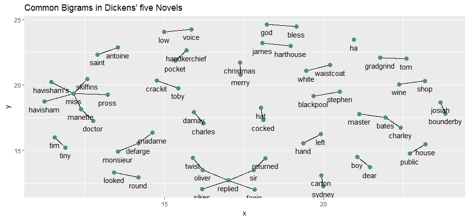
Wow, that was so much fun! I don’t want to finish as yet. I want to look into one of these five novels - “A Tale of Two Cities”.
This time I will download the plain text file for “A Tale of Two Cities” only, leave out the Project Gutenberg header and footer information, then concatenate these lines into paragraphs as following:
library(readr)
library(stringr)
raw_tale <- read_lines("ta98-0.txt", skip = 30, n_max = 15500)
tale <- character()
for (i in seq_along(raw_tale)) {
        if (i%%10 == 1) tale[ceiling(i/10)] <- str_c(raw_tale[i],
                                                     raw_tale[i+1],
                                                     raw_tale[i+2],
                                                     raw_tale[i+3],
                                                     raw_tale[i+4],
                                                     raw_tale[i+5],
                                                     raw_tale[i+6],
                                                     raw_tale[i+7],
                                                     raw_tale[i+8],
                                                     raw_tale[i+9], sep = " ")
}tale[9:10]##[1] "I. The Period It was the best of times, it was the worst of times, it ##was the age of wisdom, it was the age of foolishness, it was the epoch of ##belief, it was the epoch of incredulity, it was the season of Light," ##[2] "it was the season of Darkness, it was the spring of hope, it was the ##winter of despair, we had everything before us, we had nothing before us, we ##were all going direct to Heaven, we were all going direct the other way-- in ##short, the period was so far like the present period, that some of its ##noisiest authorities insisted on its being received, for good or for evil, ##in the superlative degree of comparison only."Sentiment in “A Tale of Two Cities”
Apply NRC sentiment dictionary to this novel.
library(syuzhet)
tale_nrc <- cbind(linenumber = seq_along(tale), get_nrc_sentiment(tale))
Create a data frame combine the line number of the book with the sentiment score, then extract positive and negative scores for visualization.
tale_nrc$negative <- -tale_nrc$negative
pos_neg <- tale_nrc %>% select(linenumber, positive, negative) %>%
        melt(id = "linenumber")
names(pos_neg) <- c("linenumber", "sentiment", "value")library(ggthemes)
ggplot(data = pos_neg, aes(x = linenumber, y = value, fill = sentiment)) +
geom_bar(stat = 'identity', position = position_dodge()) + theme_minimal() +
ylab("Sentiment") +
ggtitle("Positive and Negative Sentiment in A Tale of Two Cities") +
scale_color_manual(values = c("orange", "blue")) +
scale_fill_manual(values = c("orange", "blue"))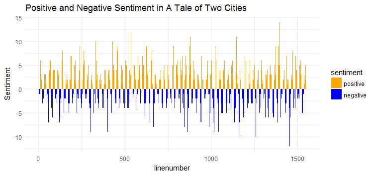
Seems the positive scores and the negative scores are almost equal overall, it does make sense given the content of the novel.
emotions <- tale_nrc %>% select(linenumber, anger, anticipation,
                                      disgust, fear, joy, sadness, surprise,
                                      trust) %>%
        melt(id = "linenumber")
names(emotions) <- c("linenumber", "sentiment", "value")
emotions_group <- group_by(emotions, sentiment)
by_emotions <- summarise(emotions_group,
                         values=sum(value))
ggplot(aes(reorder(x=sentiment, values), y=values, fill=sentiment), data = by_emotions) +
  geom_bar(stat = 'identity') + ggtitle('Sentiment in A Tale of Two Cities') +
  coord_flip() + theme(legend.position="none")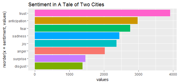
The End
Again, that was so much fun, my post just touched a bit of it on text mining. There are many more things to do such as comparing text across different novelists, save it to the next time.
Source code that created this post can be found here. I am happy to hear any feedback and questions.
References: