
Introduction
Hacker News is one of my favorite sites to catch up on technology and startup news, but navigating the minimalistic website can be sometimes tedious. Therefore, my plan in this post is to introduce you that how this social news site can be analyzed, in as non-technical a fashion as I can, as well as presenting some initial results, along with some ideas about where we will take it next.
To avoid dealing with SQL, I downloaded Hacker News dataset from David Robinson’s website, it includes one million Hacker News article titles from September 2013 to June 2017.
To begin, let’s look at the visualization of the most common words in Hacker News titles.
library(tidyverse)
library(lubridate)
library(tidytext)
library(stringr)
library(ggplot2)
library(ggthemes)
library(reshape2)
library(wordcloud)
library(tidyr)
library(igraph)
library(ggraph)
hackernews <- read_csv("stories_1000000.csv.gz") %>%
mutate(time = as.POSIXct(time, origin = "1970-01-01"),
month = round_date(time, "month"))Some initial simple exploration
Before we get into the statistical analysis, the first step is to look at the most frequent words that appeared on Hacker News titles from September 2013 to June 2017.
hackernews %>%
  unnest_tokens(word, title) %>%
  anti_join(stop_words) %>%
  count(word, sort=TRUE) %>%
  filter(n > 8000) %>%
  mutate(word = reorder(word, n)) %>%
  ggplot(aes(word, n)) +
  geom_col() +
  xlab(NULL) +
  coord_flip() +
  labs(title = "The Most Common Words in Hacker News Titles") +
  theme_fivethirtyeight()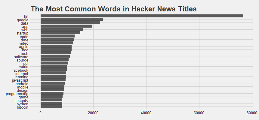
For the most part, we would expect it is a fairly standard list of common words in Hacker News titles. The top word is “hn”, because “ask hn”, “show hn” are part of the social news site’s structure. The second most frequent words such as “google”, “data”, “app”, “web”, “startup” and so on are all within our expectation for a social news site like Hacker News.
tidy_hacker <- hackernews %>%
  unnest_tokens(word, title) %>%
  anti_join(stop_words)

tidy_hacker %>%
  count(word, sort = TRUE)
### A tibble: 176,672 x 2
## word n
## <chr> <int>
## 1 hn 76530
## 2 google 23574
## 3 data 22520
## 4 app 19452
## 5 web 16075
## 6 startup 15021
## 7 code 12854
## 8 time 12656
## 9 video 12370
##10 apple 11780
### ... with 176,662 more rowsSimple Sentiment Analysis
Let’s address the topic of sentiment analysis. Sentiment analysis detects the sentiment of a body of text in terms of polarity (positive or negative). When used, particularly at scale, it can show you how people feel towards the topics that are important to you.
We can analyze word counts that contribute to each sentiment. From the Hacker news articles, We fount out how much each word contributed to each sentiment
bing_word_counts <- tidy_hacker %>%
  inner_join(get_sentiments("bing")) %>%
  count(word, sentiment, sort = TRUE) %>%
  ungroup()
bing_word_counts
### A tibble: 4,821 x 3
## word sentiment n
## <chr> <chr> <int>
## 1 free positive 11777
## 2 cloud negative 7010
## 3 top positive 5654
## 4 support positive 4805
## 5 fast positive 3604
## 6 smart positive 3266
## 7 swift positive 3247
## 8 bad negative 3234
## 9 easy positive 3216
##10 hack negative 3020
### ... with 4,811 more rowsbing_word_counts %>%
group_by(sentiment) %>%
top_n(10) %>%
ungroup() %>%
mutate(word = reorder(word, n)) %>%
ggplot(aes(word, n, fill = sentiment)) +
geom_col(show.legend = FALSE) +
facet_wrap(~sentiment, scales = "free_y") +
labs(title = "The Most Common Positive and Negative Words in Hacker News Titles", y = "Words Contribute to sentiment", x = NULL) +
coord_flip() + theme_fivethirtyeight()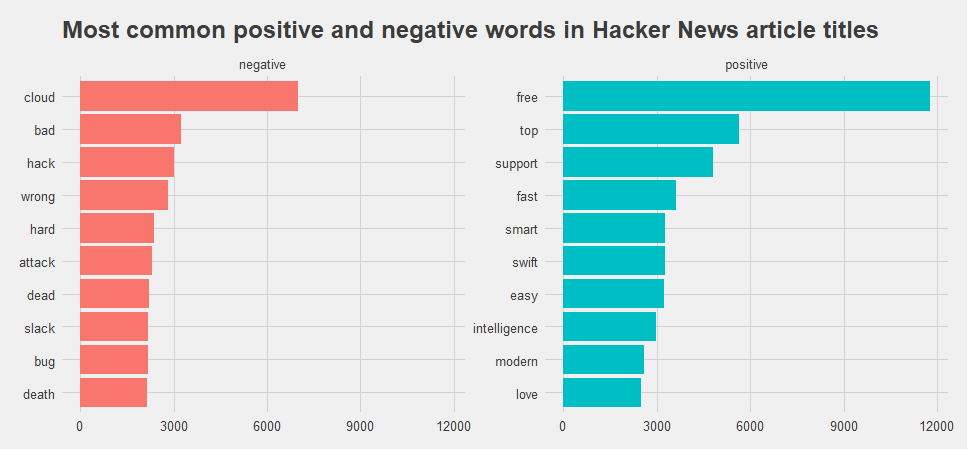
Word cloud is always a good idea to identify trends and patterns that would otherwise be unclear or difficult to see in a tabular format. We can also compare most frequent positive and negative words in word cloud.
tidy_hacker %>%
  inner_join(get_sentiments("bing")) %>%
  count(word, sentiment, sort = TRUE) %>%
  acast(word ~ sentiment, value.var = "n", fill = 0) %>%
  comparison.cloud(colors = c("#F8766D", "#00BFC4"),
                   max.words = 100)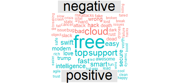
Relationship between words
we often want to understand the relationship between words in a document. What sequences of words are common across text? Given a sequence of words, what word is most likely to follow? What words have the strongest relationship with each other? Therefore, many interesting text analysis are based on the relationships. When we exam pairs of two consecutive words, it is often called “bigrams”
hacker_bigrams <- hackernews %>%
  unnest_tokens(bigram, title, token = "ngrams", n = 2)

bigrams_separated <- hacker_bigrams %>%
  separate(bigram, c("word1", "word2"), sep = " ")
bigrams_filtered <- bigrams_separated %>%
  filter(!word1 %in% stop_words$word) %>%
  filter(!word2 %in% stop_words$word)
bigram_counts <- bigrams_filtered %>%
  count(word1, word2, sort = TRUE)
bigram_counts
### A tibble: 1,255,379 x 3
## word1 word2 n
## <chr> <chr> <int>
## 1 machine learning 3369
## 2 silicon valley 3338
## 3 deep learning 2226
## 4 real time 2116
## 5 social media 1810
## 6 data science 1621
## 7 programming language 1601
## 8 raspberry pi 1584
## 9 artificial intelligence 1549
##10 san francisco 1490
### ... with 1,255,369 more rowsbigrams_united <- bigrams_filtered %>%
unite(bigram, word1, word2, sep = " ")
bigram_tf_idf <- bigrams_united %>%
count(bigram)
bigram_tf_idf <- bigram_tf_idf %>% filter(n>1000)
ggplot(aes(x = reorder(bigram, n), y=n), data=bigram_tf_idf) + geom_bar(stat = 'identity') + labs(title = "The Most Common Bigrams in Hacker News") + coord_flip() + theme_fivethirtyeight()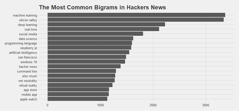
Winner of most common bigram in Hacker news data goes to “machine learning” and the second is “silicon valley”.
The challenge in analyzing text data, as mentioned earlier, is in understanding what the words mean. The use of the word “deep” has different meaning if it is paired with the word “water” as opposed to the word “learning”. As a result, a simple summary of word counts in text data will likely be confusing unless the analysis relate it to the other words that also appear without assuming an independent process of word choice.
bigram_graph <- bigram_counts %>%
  filter(n > 600) %>%
  graph_from_data_frame()
bigram_graph
##IGRAPH DN-- 76 46 --
##+ attr: name (v/c), n (e/n)
##+ edges (vertex names):
## [1] machine ->learning silicon ->valley deep ->learning
## [4] real ->time social ->media data ->science
## [7] programming->language raspberry ->pi artificial ->intelligence
##[10] san ->francisco windows ->10 hacker ->news
##[13] command ->line elon ->musk net ->neutrality
##[16] virtual ->reality app ->store mobile ->app
##[19] apple ->watch source ->code react ->native
##[22] computer ->science wi ->fi chrome ->extension
##+ ... omitted several edgesNetworks of words
Words networks analysis is one method for encoding the relationships between words in a text and constructing a network of the linked words. This technique is based on the assumption that language and knowledge can be modeled as networks of words and the relations between them.
For Hacker news data, we can visualize some details of the text structure. For example, we can see pairs or triplets that form common short phrases (“Social media network” or “neural networks”).
set.seed(2017)
ggraph(bigram_graph, layout = "fr") +
  geom_edge_link() +
  geom_node_point(color = "plum4", size = 5) +
  geom_node_text(aes(label = name), vjust = 1.8) + labs(title = "Word Network in Hacker News Dataset Titles") +
  theme_fivethirtyeight()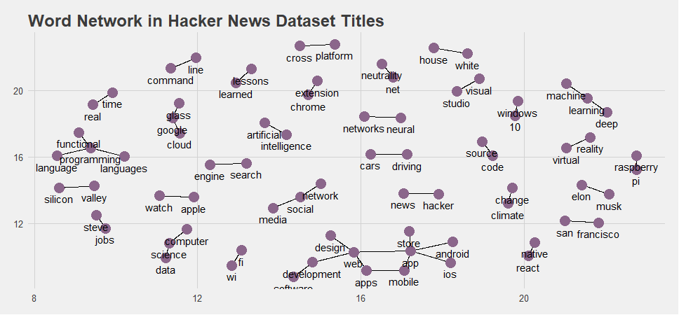
This type of network analysis is mainly showing us the important nouns in a text, and how they are related. The resulting graph can be used to get a quick visual summary of the text, read the most relevant excerpts.
Once we have the capability to automatically derive insights from text analytics, they then can translate the insights into actions.
There is no structured survey data does a better job predicting customer behavior as well as actual voice of customer text comments and messages!
Code that created this post can be found here. I welcome your comments and questions!