Text Analysis with Term Frequency for Mark Twain's Novels

Introduction

Samuel Langhorne Clemens, otherwise known as Mark Twain, is one of the most important American writers.”The Adventures of Tom Sawyer” is probably one of my most favorite books in all English literature. Happy to see that Twain’s river novels remain required reading for young students, he is read more widely now than ever!

Project Gutenberg offers over 53,000 free books. I will use four of Twain’s best novels for this analysis:

Roughing It
Life on the Mississippi
The Adventures of Tom Sawyer
Adventures of Huckleberry Finn

We will be using the following packages for the analysis:

library(tidyverse)
library(tidyr)
library(ggplot2) 
library(tidytext)
library(stringr)
library(dplyr)
library(tm)
library(topicmodels)
library(gutenbergr)
theme_set(theme_minimal())

Data preprocessing

We’ll retrieve these four books using the gutenbergr package:

books <- gutenberg_download(c(3177, 245, 74, 76), meta_fields = "title")

An important preprocessing step is tokenization. This is the process of splitting a text into individual words or sequences of words. The unnest_tokens function is a way to do just that. The result is converting the text column to be one-token-per-row like so:

tidy_books <- books %>%
  unnest_tokens(word, text)

tidy_books

### A tibble: 502,799 x 3
##   gutenberg_id                        title       word
##          <int>                        <chr>      <chr>
## 1           74 The Adventures of Tom Sawyer        the
## 2           74 The Adventures of Tom Sawyer adventures
## 3           74 The Adventures of Tom Sawyer         of
## 4           74 The Adventures of Tom Sawyer        tom
## 5           74 The Adventures of Tom Sawyer     sawyer
## 6           74 The Adventures of Tom Sawyer         by
## 7           74 The Adventures of Tom Sawyer       mark
## 8           74 The Adventures of Tom Sawyer      twain
## 9           74 The Adventures of Tom Sawyer     samuel
##10           74 The Adventures of Tom Sawyer  langhorne
# ... with 502,789 more rows

After removing stop words, we can find the most common words in all the four books as a whole.

data("stop_words")
cleaned_books <- tidy_books %>%
  anti_join(stop_words)

cleaned_books %>%
  count(word, sort = TRUE)

### A tibble: 21,630 x 2
##      word     n
##     <chr> <int>
## 1    time  1215
## 2     tom   982
## 3     day   701
## 4   river   684
## 5   night   562
## 6 hundred   490
## 7   water   483
## 8    head   471
## 9 chapter   465
##10  people   461
# ... with 21,620 more rows

Sentiment

Sentiment analysis is not the focus today, but since we are here already, why not have a quick look?

bing <- get_sentiments("bing")
bing_word_counts <- tidy_books %>%
  inner_join(bing) %>%
  count(word, sentiment, sort = TRUE) %>%
  ungroup()

bing_word_counts

### A tibble: 3,023 x 3
##     word sentiment     n
##    <chr>     <chr> <int>
## 1   well  positive   989
## 2   like  positive   856
## 3   good  positive   751
## 4  right  positive   566
## 5  great  positive   427
## 6 enough  positive   367
## 7   dead  negative   344
## 8   work  positive   311
## 9 pretty  positive   280
##10 better  positive   244
# ... with 3,013 more rows

bing_word_counts %>%
  filter(n > 100) %>%
  mutate(n = ifelse(sentiment == 'negative', -n, n)) %>%
  mutate(word = reorder(word, n)) %>%
  ggplot(aes(word, n, fill = sentiment)) +
  geom_bar(stat = 'identity') +
  theme(axis.text.x = element_text(angle = 90, hjust = 1)) +
  ylab('Contribution to sentiment') + ggtitle('Most common positive and negative words')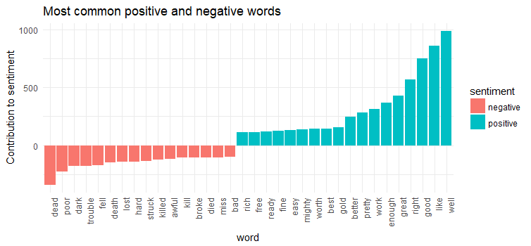

twain-1

We did not spot anomaly in the sentiment analysis results except word “miss’ is identified as a negative word, actually, it is used as a title for the tough old spinster Miss Watson in “Adventures of Huckleberry Finn”.

tf-idf

To blatantly quote the Wikipedia article on tf-idf:

In text analysis, tf-idf, short for term frequency–inverse document frequency, is a numerical statistic that is intended to reflect how important a word is to a document in a collection or corpus. It is often used as a weighting factor in information retrieval and text mining.

For our purpose, we want to know the most important words(highest tf-idf) in Mark Twain’s four books overall, and most important words(highest tf-idf) in each of these four books. Let’s find out.

book_words <- cleaned_books %>%
  count(title, word, sort = TRUE) %>%
  ungroup()

total_words <- book_words %>% 
  group_by(title) %>% 
  summarize(total = sum(n))

book_words <- left_join(book_words, total_words)

book_words

### A tibble: 38,346 x 4
##                            title   word     n total
##                            <chr>  <chr> <int> <int>
## 1   The Adventures of Tom Sawyer    tom   722 24977
## 2        Life on the Mississippi  river   486 51875
## 3        Life on the Mississippi   time   355 51875
## 4 Adventures of Huckleberry Finn    jim   351 32959
## 5                    Roughing It   time   344 62611
## 6 Adventures of Huckleberry Finn   time   325 32959
## 7                    Roughing It    day   300 62611
## 8 Adventures of Huckleberry Finn warn't   290 32959
## 9 Adventures of Huckleberry Finn     de   252 32959
##10        Life on the Mississippi  water   245 51875
# ... with 38,336 more rows

Terms with the highest tf-idf across all the four novels

book_words <- book_words %>%
  bind_tf_idf(word, title, n)

book_words %>%
  select(-total) %>%
  arrange(desc(tf_idf))

### A tibble: 38,346 x 6
##                  title   word     n          tf       idf      tf_idf
##                            <chr>  <chr> <int>       <dbl>     <dbl>       ##<dbl>
## 1 The Adventures of Tom Sawyer becky 102 0.004083757 0.6931472 0.002830645
## 2 The Adventures of Tom Sawyer tom's 97  0.003883573 0.6931472 0.002691888
## 3 The Adventures of Tom Sawyer huck  232 0.009288545 0.2876821 0.002672148
## 4 AdventuresofHuckleberry Finn warn't290 0.008798811 0.2876821 0.002531260
## 5 Life on the Mississippi     pilots  93 0.001792771 1.3862944 0.002485308
## 6 AdventuresofHuckleberry Finn dey    59 0.001790103 1.3862944 0.002481609
## 7 The Adventures of Tom Sawyer potter 44 0.001761621 1.3862944 0.002442125
## 8 AdventuresofHuckleberry Finn de    252 0.007645863 0.2876821 0.002199578
## 9 Roughing It                don’t    98 0.001565220 1.3862944 0.00216985
##10 The Adventures of Tom Sawyer sid    77 0.003082836 0.6931472 0.002136859
### ... with 38,336 more rows

plot <- book_words %>%
  arrange(desc(tf_idf)) %>%
  mutate(word = factor(word, levels = rev(unique(word))))

plot %>% 
  top_n(20) %>%
  ggplot(aes(word, tf_idf, fill = title)) +
  geom_bar(stat = 'identity', position = position_dodge())+
  labs(x = NULL, y = "tf-idf") +
  coord_flip() + ggtitle("Top tf-idf words in Mark Twain's Four Novels")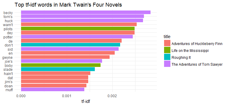

twain-2

plot %>% 
  group_by(title) %>% 
  top_n(10) %>% 
  ungroup %>%
  ggplot(aes(word, tf_idf, fill = title)) +
  geom_col(show.legend = FALSE) +
  labs(x = NULL, y = "tf-idf") +
  facet_wrap(~title, ncol = 2, scales = "free") +
  coord_flip() + ggtitle('Top tf-idf words in each novel')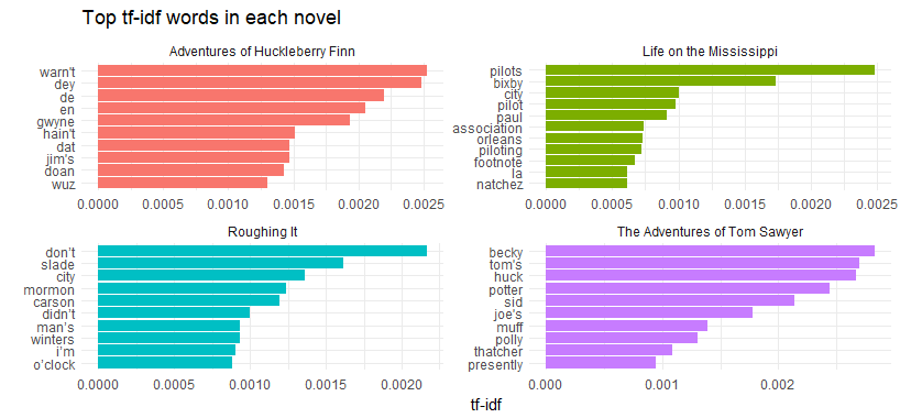

twain-3

Each novel has its own highest tf-idf words. However, the language he used across these four novels are pretty similar, such as term “city” has high tf-idf in “Roughing it” and “Life on the Mississippi”.

Term frequency

Just for the kicks, let’s compare Mark Twain’s works with those of Charles Dicken’s. Let’s get “A Tale of Two Cities”, “Great Expectations”, “A Christmas Carol in Prose; Being a Ghost Story of Christmas”, “Oliver Twist” and “Hard Times”.

What are the most common words in these novels of Charles Dickens?

dickens <- gutenberg_download(c(98, 1400, 46, 730, 786))
tidy_dickens <- dickens %>%
  unnest_tokens(word, text) %>%
  anti_join(stop_words)
tidy_dickens %>%
  count(word, sort = TRUE)

### A tibble: 19,634 x 2
##     word     n
##    <chr> <int>
## 1   time  1218
## 2   hand   918
## 3  night   835
## 4 looked   814
## 5   head   813
## 6 oliver   766
## 7   dear   751
## 8    joe   718
## 9   miss   702
##10    sir   697
### ... with 19,624 more rows

tidy_twains <- books %>%
  unnest_tokens(word, text) %>%
  anti_join(stop_words)

frequency <- bind_rows(mutate(tidy_twains, author = "Mark Twain"),
                       mutate(tidy_dickens, author = "Charles Dickens")) %>% 
  mutate(word = str_extract(word, "[a-z']+")) %>%
  count(author, word) %>%
  group_by(author) %>%
  mutate(proportion = n / sum(n)) %>% 
  select(-n) %>% 
  spread(author, proportion) %>% 
  gather(author, proportion, `Mark Twain`:`Charles Dickens`)

frequency$word <- factor(frequency$word, 
                     levels=unique(with(frequency, 
                                 word[order(proportion, word, 
                                            decreasing = TRUE)])))
frequency <- frequency[complete.cases(frequency), ]
ggplot(aes(x = reorder(word, proportion), y = proportion, fill = author), 
       data = subset(frequency, proportion>0.0025)) +
  geom_bar(stat = 'identity', position = position_dodge())+
  coord_flip() + ggtitle('Comparing the word frequencies of Mark Twain and Charles Dickens')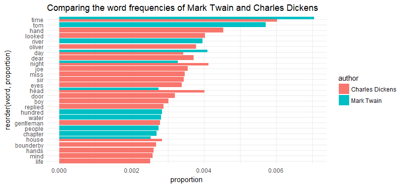

twain-4

The top term for both author is the same - “time”. Other than that, their language are very different.

Susan Li

My Favorite Blogs

Text Analysis with Term Frequency for Mark Twain's Novels

Introduction

Data preprocessing

Sentiment

tf-idf

Term frequency

Susan Li

My Favorite Blogs

Text Analysis with Term Frequency for Mark Twain's Novels

Introduction

Data preprocessing

Sentiment

tf-idf

Term frequency

You might also enjoy (View all posts)