Setup
This project details our analysis of the movie dataset that contains information from Rotten Tomatos and IMDB for a random sample of movies. The purpose of this project is to develop a multiple linear regression model to understand what attributes make a movie popular. In the meantime, learning something new about movies.
Load packages
library(ggplot2)
library(dplyr)
library(statsr)
library(gridExtra)
library(corrplot)
Load data
load("movies.Rdata")Part 1: Data
The data set is comprised of 651 randomly sampled movies produced and released before 2016, each row in the dataset is a movie and each column is a characteristic of a movie. Therefore, the data should allow us to generalize to the population of interest. However, there is no causation can be established because random assignment is not used in this study. In addition, potential biases are associated with non-voting or non_rating because the voting and rating are voluntary on IMDB and Rotten Tomatos website.
From common sense, we realized that many of the variables are irrelevant to the purpose of identifying the popularity of a movie. As such, we select the following variables to start our analysis.
- title_type: Type of movie (Documentary, Feature Film, TV Movie)
- genre: Genre of movie (Action & Adventure, Comedy, Documentary, Drama, Horror, Mystery & Suspense, Other)
- runtime: Runtime of movie (in minutes)
- imdb_rating: Rating on IMDB
- imdb_num_votes: Number of votes on IMDB
- critics_rating: Categorical variable for critics rating on Rotten Tomatoes (Certified Fresh, Fresh, Rotten)
- critics_score: Critics score on Rotten Tomatoes
- audience_rating: Categorical variable for audience rating on Rotten Tomatoes (Spilled, Upright)
- audience_score: Audience score on Rotten Tomatoes
- best_pic_win: Whether or not the movie won a best picture Oscar (no, yes)
- best_actor_win: Whether or not one of the main actors in the movie ever won an Oscar (no, yes) - note that this is not necessarily whether the actor won an Oscar for their role in the given movie
- best_actress win: Whether or not one of the main actresses in the movie ever won an Oscar (no, yes) - not that this is not necessarily whether the actresses won an Oscar for their role in the given movie
- best_dir_win: Whether or not the director of the movie ever won an Oscar (no, yes) - not that this is not necessarily whether the director won an Oscar for the given movie
Part 2: Research question
Is a movie’s popularity, as measured by audience score, related to the type of movie, genre, runtime, imdb rating, imdb number of votes, critics rating, critics score, audience rating, Oscar awards obtained (actor, actress, director and picture)? Being able to answer this question will help us to predict a movie’s popularity.
Part 3: Exploratory data analysis and feature selection
Abstracting the data of the above potential predictors for the model.
movies_new <- movies %>% select(title, title_type, genre, runtime, imdb_rating, imdb_num_votes, critics_rating, critics_score, audience_rating, audience_score, best_pic_win, best_actor_win, best_actress_win, best_dir_win)Look at the structure of the data
str(movies_new)##Classes 'tbl_df', 'tbl' and 'data.frame': 650 obs. of 14 variables:
## $ title : chr "Filly Brown" "The Dish" "Waiting for Guffman" ##"The Age of Innocence" ...
## $ title_type : Factor w/ 3 levels "Documentary",..: 2 2 2 2 2 1 2 2 1 ##2 ...
## $ genre : Factor w/ 11 levels "Action & Adventure",..: 6 6 4 6 7 ##5 6 6 5 6 ...
## $ runtime : num 80 101 84 139 90 78 142 93 88 119 ...
## $ imdb_rating : num 5.5 7.3 7.6 7.2 5.1 7.8 7.2 5.5 7.5 6.6 ...
## $ imdb_num_votes : int 899 12285 22381 35096 2386 333 5016 2272 880 12496 ##...
## $ critics_rating : Factor w/ 3 levels "Certified Fresh",..: 3 1 1 1 3 2 3 ##3 2 1 ...
## $ critics_score : num 45 96 91 80 33 91 57 17 90 83 ...
## $ audience_rating : Factor w/ 2 levels "Spilled","Upright": 2 2 2 2 1 2 2 1 ##2 2 ...
## $ audience_score : num 73 81 91 76 27 86 76 47 89 66 ...
## $ best_pic_win : Factor w/ 2 levels "no","yes": 1 1 1 1 1 1 1 1 1 1 ...
## $ best_actor_win : Factor w/ 2 levels "no","yes": 1 1 1 2 1 1 1 2 1 1 ...
## $ best_actress_win: Factor w/ 2 levels "no","yes": 1 1 1 1 1 1 1 1 1 1 ...
## $ best_dir_win : Factor w/ 2 levels "no","yes": 1 1 1 2 1 1 1 1 1 1 ...
## - attr(*, "na.action")=Class 'omit' Named int 334
## .. ..- attr(*, "names")= chr "334"Summary statistics
summary(movies_new)## title title_type genre runtime
## Length:650 Documentary : 54 Drama :305 Min. : 39.0
## Class :character Feature Film:591 Comedy : 87 1st Qu.: 92.0
## Mode :character TV Movie :5 Action & Adventure: 65 Median :103.0
## Mystery & Suspense: 59 Mean :105.8
## Documentary : 51 3rd Qu.:115.8
## Horror : 23 Max. :267.0
## (Other) : 60
## imdb_rating imdb_num_votes critics_rating critics_score
## Min. :1.900 Min. : 180 Certified Fresh:135 Min. : 1.00
## 1st Qu.:5.900 1st Qu.: 4584 Fresh :208 1st Qu.: 33.00
## Median :6.600 Median : 15204 Rotten :307 Median : 61.00
## Mean :6.492 Mean : 57620 Mean : 57.65
## 3rd Qu.:7.300 3rd Qu.: 58484 3rd Qu.: 83.00
## Max. :9.000 Max. :893008 Max. :100.00
## audience_rating audience_score best_pic_win best_actor_win ##best_actress_win
## Spilled:275 Min. :11.00 no :643 no :557 no :578
## Upright:375 1st Qu.:46.00 yes: 7 yes: 93 yes: 72
## Median :65.00
## Mean :62.35
## 3rd Qu.:80.00
## Max. :97.00
## best_dir_win
## no :607
## yes: 43 I find there is one missing value, and decide to drop it.
movies_new <- na.omit(movies_new)Part of this project is to use the model to predict a movie’s audience score and this movie should not be part of the data. Therefore, I split the data into traning and testing, and there is only one row in the test set.
set.seed(2017)
split <- sample(seq_len(nrow(movies_new)), size = floor(0.999 * nrow(movies_new)))
train <- movies_new[split, ]
test <- movies_new[-split, ]
dim(train)
##[1] 649 14dim(test)##[1] 1 14Histogram of Numeric variables
hist(train$audience_score)
summary(train$audience_score)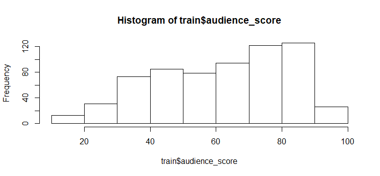
## Min. 1st Qu.  Median    Mean 3rd Qu.    Max.
## 11.0    46.0    65.0    62.3    80.0    97.0
The median of our response variable - audience score distribution is 65; 25% of the movie in the training set have an audience score higher than 80; 25% of the movie in the training set have an audience score lower than 46; very few movie have an audience score lower than 20 or higher than 90 (i.e.Audience in the data are unlikey to give very low or very high score).
p1 <- ggplot(aes(x=runtime), data=train) +
  geom_histogram(aes(y=100*(..count..)/sum(..count..)), color='black', fill='white', binwidth = 5) + ylab('percentage') + ggtitle('Run Time')
p2 <- ggplot(aes(x=imdb_rating), data=train) +
  geom_histogram(aes(y=100*(..count..)/sum(..count..)), color='black', fill='white', binwidth = 0.2) + ylab('percentage') + ggtitle('IMDB rating')
p3 <- ggplot(aes(x=log10(imdb_num_votes)), data=train) +
  geom_histogram(aes(y=100*(..count..)/sum(..count..)), color='black', fill='white') + ylab('percentage') + ggtitle('log(IMDB number of votes)')
p4 <- ggplot(aes(x=critics_score), data=train) +
  geom_histogram(aes(y=100*(..count..)/sum(..count..)), color='black', fill='white', binwidth = 2) + ylab('percentage') + ggtitle('Critics Score')
grid.arrange(p1, p2, p3, p4, ncol=2)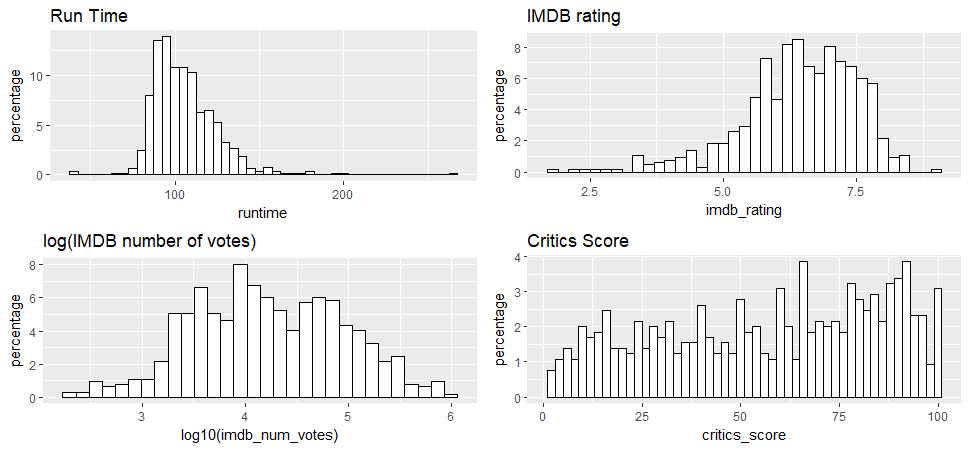
Regression analysis: Run time, IMDB rating, log(IMDB number of votes) and Critics Scores all have reasonable broad distribution, therefore, they will be considered for the regression analysis.
Bar plot of categorical variables
p1 <- ggplot(aes(x=title_type), data=train) + geom_bar(aes(y=100*(..count..)/sum(..count..))) + ylab('percentage') +
  ggtitle('Title Type') + coord_flip()
p2 <- ggplot(aes(x=genre), data=train) + geom_bar(aes(y=100*(..count..)/sum(..count..))) + ylab('percentage') +
  ggtitle('Genre') + coord_flip()
p3 <- ggplot(aes(x=critics_rating), data=train) + geom_bar(aes(y=100*(..count..)/sum(..count..))) + ylab('percentage') +
  ggtitle('Critics Rating') + coord_flip()
p4 <- ggplot(aes(x=audience_rating), data=train) + geom_bar(aes(y=100*(..count..)/sum(..count..))) + ylab('percentage') +
  ggtitle('Audience Rating') + coord_flip()
grid.arrange(p1, p2, p3, p4, ncol=2)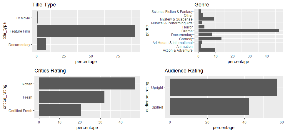
Not all those categorical variables have reasonable spread of distribution. Most movies in the data are in the “Feature Film” title type and majority of the movies are drama. Therefore, we must be aware that the results could be biased toward drama movies.
Correlation between numerical variables
vars <- names(train) %in% c('runtime', 'imdb_rating', 'imdb_num_votes', 'critics_score')
selected_train <- train[vars]
corr.matrix <- cor(selected_train)
corrplot(corr.matrix, main="\n\nCorrelation Plot of numerical variables", method="number")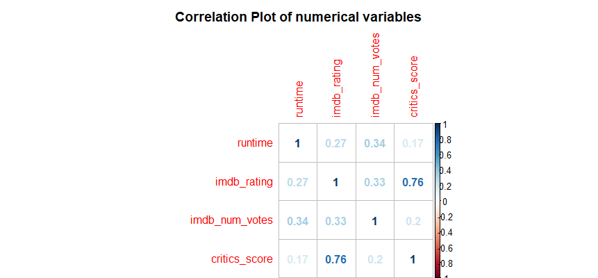
Two predictors - critics score and imdb rating are highly correlated at 0.76 (collinearity), therefore, One of them will be removed from the model, I decided to remove critics score.
Correlation between categorical variables and audience score
boxplot(audience_score~critics_rating, data=train, main='Audience score vs. Critics rating', xlab='Critics Rating', ylab='Audience Score')
by(train$audience_score, train$critics_rating, summary)
boxplot(audience_score~audience_rating, data=train, main='Audience Score vs. Audience Rating', xlab='Audience rating', ylab='Audience Score')
by(train$audience_score, train$audience_rating, summary)
boxplot(audience_score~title_type, data=train, main='Audience score vs. Title type', xlab='Title_type', ylab='Audience Score')
by(train$audience_score, train$title_type, summary)
boxplot(audience_score~genre, data=train, main='Audience score vs. Genre', xlab='Genre', ylab='Audience score')
by(train$audience_score, train$genre, summary)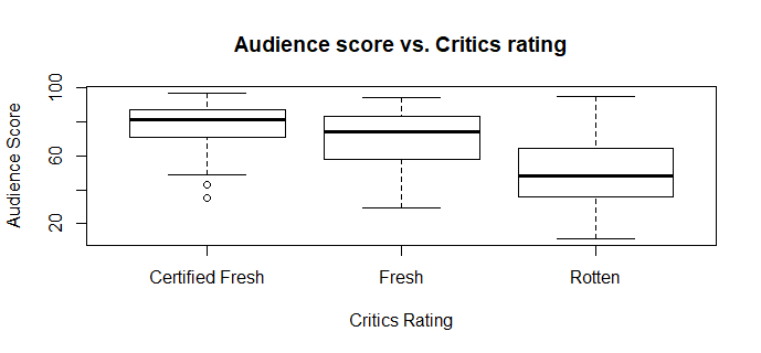
##train$critics_rating: Certified Fresh
##   Min. 1st Qu.  Median    Mean 3rd Qu.    Max.
##  35.00   71.00   81.00   79.26   87.00   97.00
##--------------------------------------------------------------
##train$critics_rating: Fresh
##   Min. 1st Qu.  Median    Mean 3rd Qu.    Max.
##  29.00   58.00   74.00   69.96   83.00   94.00
##--------------------------------------------------------------
##train$critics_rating: Rotten
##   Min. 1st Qu.  Median    Mean 3rd Qu.    Max.
##   11.0    36.0    48.0    49.7    64.0    95.0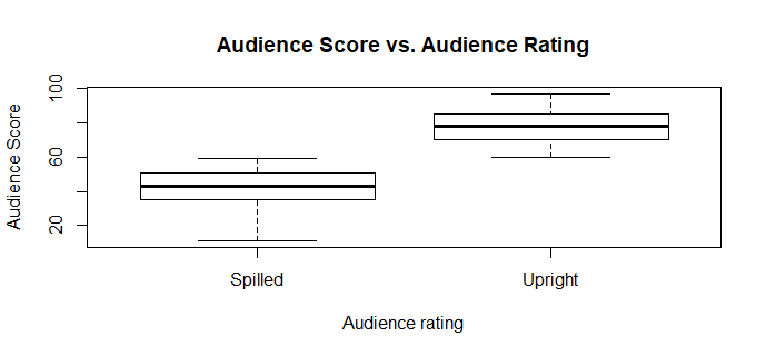
##train$audience_rating: Spilled
##   Min. 1st Qu.  Median    Mean 3rd Qu.    Max.
##  11.00   35.00   43.00   41.93   51.00   59.00
##--------------------------------------------------------------
##train$audience_rating: Upright
##   Min. 1st Qu.  Median    Mean 3rd Qu.    Max.
## 60.00 70.00 78.00 77.27 85.00 97.00 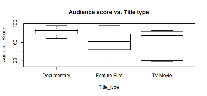
##train$title_type: Documentary
##   Min. 1st Qu.  Median    Mean 3rd Qu.    Max.
##  68.00   78.00   86.00   83.46   89.00   96.00
##--------------------------------------------------------------
##train$title_type: Feature Film
##   Min. 1st Qu.  Median    Mean 3rd Qu.    Max.
##  11.00   44.25   62.00   60.41   78.00   97.00
##--------------------------------------------------------------
##train$title_type: TV Movie
##   Min. 1st Qu.  Median    Mean 3rd Qu.    Max.
## 19.0 21.0 75.0 56.8 83.0 86.0 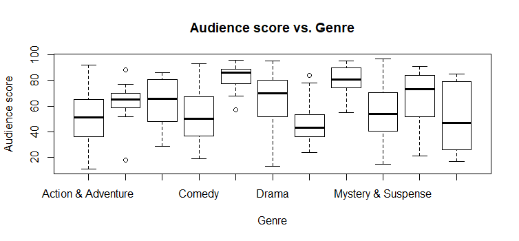
##train$genre: Action & Adventure
##   Min. 1st Qu.  Median    Mean 3rd Qu.    Max.
##  11.00   36.50   51.50   53.16   65.00   92.00
##--------------------------------------------------------------
##train$genre: Animation
##   Min. 1st Qu.  Median    Mean 3rd Qu.    Max.
##  18.00   59.00   65.00   62.44   70.00   88.00
##--------------------------------------------------------------
##train$genre: Art House & International
##   Min. 1st Qu.  Median    Mean 3rd Qu.    Max.
##  29.00   51.25   65.50   64.00   80.25   86.00
##--------------------------------------------------------------
##train$genre: Comedy
##   Min. 1st Qu.  Median    Mean 3rd Qu.    Max.
##  19.00   37.00   50.00   52.51   67.50   93.00
##--------------------------------------------------------------
##train$genre: Documentary
##   Min. 1st Qu.  Median    Mean 3rd Qu.    Max.
##  57.00   77.50   86.00   82.96   89.00   96.00
##--------------------------------------------------------------
##train$genre: Drama
##   Min. 1st Qu.  Median    Mean 3rd Qu.    Max.
##  13.00   52.00   70.00   65.35   80.00   95.00
##--------------------------------------------------------------
##train$genre: Horror
##   Min. 1st Qu.  Median    Mean 3rd Qu.    Max.
##  24.00   36.00   43.00   45.83   53.50   84.00
##--------------------------------------------------------------
##train$genre: Musical & Performing Arts
##   Min. 1st Qu.  Median    Mean 3rd Qu.    Max.
##  55.00   75.75   80.50   80.17   89.50   95.00
##--------------------------------------------------------------
##train$genre: Mystery & Suspense
##   Min. 1st Qu.  Median    Mean 3rd Qu.    Max.
##  15.00   40.50   54.00   55.95   70.50   97.00
##--------------------------------------------------------------
##train$genre: Other
##   Min. 1st Qu.  Median    Mean 3rd Qu.    Max.
##  21.00   53.00   73.50   66.69   82.50   91.00
##--------------------------------------------------------------
##train$genre: Science Fiction & Fantasy
##   Min. 1st Qu.  Median    Mean 3rd Qu.    Max.
##  17.00   26.00   47.00   50.89   79.00   85.00
All the categorical variables seems to have reasonable significant correlation with audience score.
Part 4: Modeling
We will be using stepwise model forward selection method, we start with an empty model, then add variables one at a time until a parsimonious model is reached. From the following full model, we can see that imdb rating has the lowest p value and is the most correlated variable to our response variable. So we choose imdb rating as the first predictor.
full_model <- lm(audience_score~imdb_rating+title_type+genre+runtime+imdb_num_votes+critics_rating+audience_rating+best_pic_win+best_actor_win+best_actress_win+best_dir_win, data=train)
summary(full_model)
##Call:
##lm(formula = audience_score ~ imdb_rating + title_type + genre +
## runtime + imdb_num_votes + critics_rating + audience_rating +
## best_pic_win + best_actor_win + best_actress_win + best_dir_win,
## data = train)
##Residuals:
## Min 1Q Median 3Q Max
##-21.5617 -4.4946 0.5783 4.3575 24.5177
##Coefficients:
## Estimate Std. Error t value Pr(>|t|)
##(Intercept) -9.973e+00 4.054e+00 -2.460 0.0142 *
##imdb_rating 9.549e+00 4.288e-01 22.271 <2e-16 ***
##title_typeFeature Film 2.223e+00 2.544e+00 0.874 0.3826
##title_typeTV Movie 6.679e-01 4.031e+00 0.166 0.8685
##genreAnimation 3.267e+00 2.478e+00 1.318 0.1879
##genreArt House & International -2.527e+00 2.063e+00 -1.225 0.2210
##genreComedy 1.563e+00 1.146e+00 1.364 0.1731
##genreDocumentary 2.550e+00 2.725e+00 0.936 0.3498
##genreDrama -5.613e-01 9.977e-01 -0.563 0.5739
##genreHorror -1.842e+00 1.688e+00 -1.091 0.2757
##genreMusical & Performing Arts 3.615e+00 2.361e+00 1.531 0.1263
##genreMystery & Suspense -3.108e+00 1.273e+00 -2.441 0.0149 *
##genreOther 3.295e-01 1.956e+00 0.168 0.8663
##genreScience Fiction & Fantasy -1.720e-01 2.462e+00 -0.070 0.9443
##runtime -2.532e-02 1.665e-02 -1.521 0.1288
##imdb_num_votes 2.719e-06 3.094e-06 0.879 0.3798
##critics_ratingFresh 1.594e-02 8.429e-01 0.019 0.9849
##critics_ratingRotten -1.197e+00 9.307e-01 -1.286 0.1989
##audience_ratingUpright 2.009e+01 7.905e-01 25.408 <2e-16 ***
##best_pic_winyes 5.692e-01 2.931e+00 0.194 0.8461
##best_actor_winyes 2.680e-01 8.128e-01 0.330 0.7417
##best_actress_winyes -1.031e+00 9.022e-01 -1.143 0.2534
##best_dir_winyes 5.604e-02 1.199e+00 0.047 0.9627
##---
##Signif. codes: 0 '***' 0.001 '**' 0.01 '*' 0.05 '.' 0.1 ' ' 1
##Residual standard error: 6.87 on 626 degrees of freedom
##Multiple R-squared: 0.8884, Adjusted R-squared: 0.8845
##F-statistic: 226.5 on 22 and 626 DF, p-value: < 2.2e-16fit1 <- lm(audience_score ~ imdb_rating, data=train)
summary(fit1)##Call:
##lm(formula = audience_score ~ imdb_rating, data = train)
##Residuals:
## Min 1Q Median 3Q Max
##-26.805 -6.548 0.647 5.678 52.907
##Coefficients:
## Estimate Std. Error t value Pr(>|t|)
##(Intercept) -42.3620 2.4269 -17.45 <2e-16 ***
##imdb_rating 16.1300 0.3689 43.72 <2e-16 ***
##---
##Signif. codes: 0 '***' 0.001 '**' 0.01 '*' 0.05 '.' 0.1 ' ' 1
##Residual standard error: 10.17 on 647 degrees of freedom
##Multiple R-squared: 0.7471, Adjusted R-squared: 0.7467
##F-statistic: 1911 on 1 and 647 DF, p-value: < 2.2e-16The 0.75 R-squared and almost zero p value indicate that imdb rating is a statistically significant predictor of audience score.
In order to find out the second predictor, I look at the following model.
fit_model <- lm(audience_score~title_type+genre+runtime+imdb_num_votes+critics_rating+audience_rating+best_pic_win+best_actor_win+best_actress_win+best_dir_win, data=train)
summary(fit_model)
##Call:
##lm(formula = audience_score ~ title_type + genre + runtime +
## imdb_num_votes + critics_rating + audience_rating + best_pic_win +
## best_actor_win + best_actress_win + best_dir_win, data = train)
##Residuals:
## Min 1Q Median 3Q Max
##-30.4266 -6.0224 0.8273 6.6292 19.4100
##Coefficients:
## Estimate Std. Error t value Pr(>|t|)
##(Intercept) 4.478e+01 4.312e+00 10.384 < 2e-16 ***
##title_typeFeature Film -8.169e-01 3.398e+00 -0.240 0.81009
##title_typeTV Movie -6.046e+00 5.377e+00 -1.124 0.26128
##genreAnimation 2.038e-01 3.310e+00 0.062 0.95091
##genreArt House & International 6.481e-01 2.753e+00 0.235 0.81395
##genreComedy 4.431e-01 1.531e+00 0.289 0.77239
##genreDocumentary 8.187e+00 3.630e+00 2.255 0.02445 *
##genreDrama 1.751e+00 1.327e+00 1.319 0.18756
##genreHorror -6.791e-01 2.257e+00 -0.301 0.76362
##genreMusical & Performing Arts 8.147e+00 3.147e+00 2.589 0.00985 **
##genreMystery & Suspense -2.891e-01 1.695e+00 -0.171 0.86462
##genreOther 6.906e-01 2.616e+00 0.264 0.79190
##genreScience Fiction & Fantasy -3.348e+00 3.288e+00 -1.018 0.30898
##runtime 2.253e-02 2.208e-02 1.020 0.30801
##imdb_num_votes 1.798e-05 4.037e-06 4.454 9.98e-06 ***
##critics_ratingFresh -3.830e-01 1.127e+00 -0.340 0.73416
##critics_ratingRotten -7.227e+00 1.191e+00 -6.067 2.25e-09 ***
##audience_ratingUpright 2.897e+01 9.128e-01 31.740 < 2e-16 ***
##best_pic_winyes -9.016e-01 3.920e+00 -0.230 0.81816
##best_actor_winyes 8.810e-01 1.087e+00 0.811 0.41787
##best_actress_winyes -5.768e-01 1.207e+00 -0.478 0.63280
##best_dir_winyes 1.256e+00 1.603e+00 0.784 0.43345
##---
##Signif. codes: 0 '***' 0.001 '**' 0.01 '*' 0.05 '.' 0.1 ' ' 1
##Residual standard error: 9.191 on 627 degrees of freedom
##Multiple R-squared: 0.7999, Adjusted R-squared: 0.7932
##F-statistic: 119.4 on 21 and 627 DF, p-value: < 2.2e-16We add audience rating as the second predictor because of the lowest p value.
fit2 <- lm(audience_score ~ imdb_rating + audience_rating, data=train)
summary(fit2)
##Call:
##lm(formula = audience_score ~ imdb_rating + audience_rating,
## data = train)
##Residuals:
## Min 1Q Median 3Q Max
##-22.1619 -4.7622 0.6187 4.3354 24.2864
##Coefficients:
## Estimate Std. Error t value Pr(>|t|)
##(Intercept) -11.4476 2.0110 -5.693 1.9e-08 ***
##imdb_rating 9.5122 0.3505 27.142 < 2e-16 ***
##audience_ratingUpright 20.8687 0.7676 27.188 < 2e-16 ***
##---
##Signif. codes: 0 '***' 0.001 '**' 0.01 '*' 0.05 '.' 0.1 ' ' 1
##Residual standard error: 6.952 on 646 degrees of freedom
##Multiple R-squared: 0.8821, Adjusted R-squared: 0.8817
##F-statistic: 2416 on 2 and 646 DF, p-value: < 2.2e-16The models’ R-squared and Adjusted R-Squared both increased significantly, the almost zero p value indicate that audience rating is another statistically significant predictor of audience score.
After the above second fit, I did the following attempts:
- Added critics rating to the model but the Adjust R-squared only increased from 0.8817 to 0.8819, the p value is insignificant at 0.61896 and 0.10116. Therefore, we will not include critics rating as a predictor.
- Added imdb_num_votes to the model but the Adjust R-squared decreased from 0.8817 to 0.8815 and the p value is not significant at 0.734. So, we will not include imdb_num_votes to the model.
- Added genre to the model and the Adjust R-squared increased from 0.8817 to 0.8847, the amount varaince it explains at 0.8868 versus 0.8812 without. From the anova analysis we can see that the p value is significant at 0.0033.
- It is obvious that title type, runtime, best_pic_win, best_actor_win, best_actress_win, best_dir_win are not significant predictors, therefore, they will not be included in the model.
fit3 <- lm(audience_score ~ imdb_rating + audience_rating + genre, data=train)
anova(fit3)
##Analysis of Variance Table
##Response: audience_score
## Df Sum Sq Mean Sq F value Pr(>F)
##imdb_rating 1 197779 197779 4198.2813 < 2.2e-16 ***
##audience_rating 1 35724 35724 758.3151 < 2.2e-16 ***
##genre 10 1259 126 2.6722 0.003309 **
##Residuals 636 29962 47
##---
##Signif. codes: 0 '***' 0.001 '**' 0.01 '*' 0.05 '.' 0.1 ' ' 1Therefore, I decide to add genre as one of the prdictors. So, I arrived at our final model - Parsimonious Model, with three predictors: imdb rating, audience rating and genre.
summary(fit3)##Call:
##lm(formula = audience_score ~ imdb_rating + audience_rating +
## genre, data = train)
##Residuals:
## Min 1Q Median 3Q Max
##-21.6679 -4.4091 0.6113 4.3309 25.0302
##Coefficients:
## Estimate Std. Error t value Pr(>|t|)
##(Intercept) -12.5142 2.1981 -5.693 1.91e-08 ***
##imdb_rating 9.7844 0.3705 26.407 < 2e-16 ***
##audience_ratingUpright 20.3246 0.7751 26.222 < 2e-16 ***
##genreAnimation 3.6812 2.4546 1.500 0.1342
##genreArt House & International -2.7199 2.0368 -1.335 0.1822
##genreComedy 1.5684 1.1320 1.386 0.1664
##genreDocumentary 0.6890 1.3789 0.500 0.6175
##genreDrama -0.7612 0.9677 -0.787 0.4318
##genreHorror -1.5608 1.6733 -0.933 0.3513
##genreMusical & Performing Arts 2.6242 2.1958 1.195 0.2325
##genreMystery & Suspense -3.2036 1.2529 -2.557 0.0108 *
##genreOther 0.3460 1.9302 0.179 0.8578
##genreScience Fiction & Fantasy 0.3138 2.4440 0.128 0.8979
##---
##Signif. codes: 0 '***' 0.001 '**' 0.01 '*' 0.05 '.' 0.1 ' ' 1
##Residual standard error: 6.864 on 636 degrees of freedom
##Multiple R-squared: 0.8868, Adjusted R-squared: 0.8847
##F-statistic: 415.3 on 12 and 636 DF, p-value: < 2.2e-16Interpretation of the model:
- Intercept(-12.5142) is the estimated audience score for a movie with imdb_rating, audience_rating and genre at zero. It does not provide any meaningful interpretation here.
- imdb_rating coefficient(9.7844): All else hold constant, for every one unit increase in imdb_rating, the model predicts a 9.7844 increase in audience_score on average.
- audience_ratingUpright coefficient(20.3246): All else hold constant, the model predicts rating Upright movie is 20.3246 higher in audience score on average than rating Spilled movie.
- genreAnimation coefficient(3.6812): The model predicts that Animation films get an audience score that is 3.6812 higher than Action & Adventure(reference category) films on average after controlling for imdb_rating and audience rating.
- genreArt House & International coefficient(-2.7199): The model predicts that Art House & International films get an audience score that is 2.7199 lower than Action & Adventure films on average after controlling for imdb_rating and audience rating.
- There are total 11 genre categories in the dataset, the audience score can higher or lower than Action & Adventure films depends on what genre is selected.
- R-Squared(0.8847): 88.47% of the variablity in audience score can be explained by the model.
Model diagnostics
ggplot(data = fit3, aes(x = .fitted, y = .resid)) +
  geom_point() +
  geom_hline(yintercept = 0, linetype = "dashed") +
  xlab("Fitted values") +
  ylab("Residuals")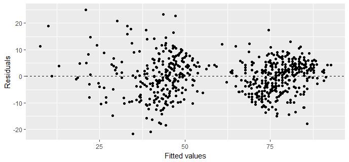
There is clear a linear relationship between imdb rating and audience score. The linearity condition is met by our model.
Constant variance of residuals condition met, No fan shape in residuals plot.
ggplot(data = fit3, aes(x = .resid)) +
  geom_histogram(binwidth = 1, fill='white', color='black') +
  xlab("Residuals")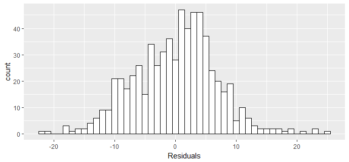
ggplot(data = fit3, aes(sample = .resid)) +
  stat_qq()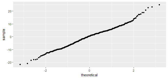
The residuals are nearly symmetric, hence it would be appropriate to deem the the normal distribution of residuals condition met.
Part 5: Prediction
We are going to use the final model(fit3) to predict the audience score for the movie in the test set - Aliens. First we create a new dataframe for this movie.
newmovie <- test %>% select(genre, imdb_rating, audience_rating)
predict(fit3, newmovie)##89.99899The model predicts movie Aliens in the test set will have an audience score at approximate 90.
predict(fit3, newmovie, interval = "prediction", level = 0.95)## fit lwr upr
##1 89.99899 76.34498 103.653Our model predicts, with 95% confidence, that the movie Aliens is expected to have an audience score between 76.34 and 103.65.
test$audience_score##[1] 94The actual audience score for this movie is 94. Our prediction interval contains this value.
Part 6: Conclusion
Our model demonstrates that it is possible to predict a movie’s popularity, as measured by audience score with only three predictors - imdb score, audience rating and genre. Movie industries can use the similar methods when producing movies that are more likely to be liked by the target audience.
However, the potential shortcoming is that our model’s predictive power is limited because the sample data is not representative. Therefore, a larger number of observations to capture more variability in the population data in our testing data set is required to have a better measure of the model’s accuracy.
