In machine learning and natural language processing, A “topic” consists of a cluster of words that frequently occur together. A topic model is a type of statistical model for discovering the abstract “topics” that occur in a collection of documents. Topic modeling is a frequently used text-mining tool for discovery of hidden semantic structures in a text body. Topic models can connect words with similar meanings and distinguish between uses of words with multiple meanings.
For this analysis, I downloaded 22 recent articles from business and technology sections at New York Times. I am using the collection of these 22 articles as my corpus for the topic modeling exercise. Therefore, each article is a document, with an unknown topic structure.
Load the library
library(tm)
library(topicmodels)
library(SnowballC)
library(tidytext)
library(ggplot2)
library(dplyr)
Set the working directory.
setwd('C:/Users/Susan/Documents/textmining')Load the files into corpus.
filenames <- list.files(getwd(),pattern='*.txt')Read the files into a character vector.
files <- lapply(filenames, readLines)Create corpus from the vector and inspect the 5th document.
docs <- Corpus(VectorSource(files))
writeLines(as.character(docs[[5]]))
##c("The Food and Drug Administration on Wednesday approved the first-ever ##treatment that genetically alters a patient’s own cells to fight cancer, a ##milestone that is expected to transform treatment in the coming years.The ##new therapy turns a patient’s cells into a “living drug,” and trains them to ##recognize and attack the disease. It is part of the rapidly growing field ##of", "immunotherapy that bolster...Data Preprocessing
Remove potential problematic symbols
toSpace <- content_transformer(function(x, pattern) {return (gsub(pattern, '', x))})
docs <- tm_map(docs, toSpace, '-')
docs <- tm_map(docs, toSpace, ':')
docs <- tm_map(docs, toSpace, '“')
docs <- tm_map(docs, toSpace, '”')
docs <- tm_map(docs, toSpace, "'")
Remove punctuation, digits, stop words and white space.
docs <- tm_map(docs, removePunctuation)
docs <- tm_map(docs, removeNumbers)
docs <- tm_map(docs, removeWords, stopwords('english'))
docs <- tm_map(docs, stripWhitespace)
Define and remove custom stop words.
myStopwords <- c('can','say','said','will','like','even','well','one', 'hour', 'also', 'take', 'well','now','new', 'use', 'the')
docs <- tm_map(docs, removeWords, myStopwords)
I decided to go further and remove everything that is not alpha or numerical symbol or space.
removeSpecialChars <- function(x) gsub("[^a-zA-Z0-9 ]","",x)
docs <- tm_map(docs, removeSpecialChars)
Transform to lowercase.
docs <- tm_map(docs, content_transformer(tolower))Stem the document. It looks right after all the preprocessing.
docs <- tm_map(docs,stemDocument)
writeLines(as.character(docs[[5]]))
##cthe food drug administr wednesday approv firstev treatment genet alter ##patient cell fight cancer mileston expect transform treatment come yearsth ##therapi turn patient cell live drug train recogn attack diseas it part rapid ##grow field immunotherapi...Right now this data frame is in a tidy form, with one-term-per-document-per-row. However, the topicmodels package requires a DocumentTermMatrix. We can create a DocumentTermMatrix like so:
dtm <- DocumentTermMatrix(docs)
dtm
##<<DocumentTermMatrix (documents: 22, terms: 3290)>>
##Non-/sparse entries: 7323/65057
##Sparsity : 90%
##Maximal term length: 18
##Weighting : term frequency (tf)Topic Modeling
Latent Dirichlet allocation (LDA) is one of the most common algorithms for topic modeling. LDA assumes that each document in a corpus contains a mix of topics that are found throughout the entire corpus. The topic structure is unknown - we can only observe the documents and words, not the topics themselves. Because the structure is unknown (also known as latent), this method seeks to infer the topic structure given the known words and documents.
Now We are ready to use the LDA() function from the topicmodels package. Let’s estimate an LDA model for these New york Times articles, setting k = 4, to create a 4-topic LDA model.
nytimes_lda <- LDA(dtm, k = 4, control = list(seed = 1234))
nytimes_lda
##A LDA_VEM topic model with 4 topics.Word-topic probabilities
nytimes_topics <- tidy(nytimes_lda, matrix = "beta")
nytimes_topics
### A tibble: 13,160 x 3
## topic term beta
## <int> <chr> <dbl>
## 1 1 adapt 3.204101e-04
## 2 2 adapt 8.591570e-103
## 3 3 adapt 1.585924e-100
## 4 4 adapt 5.643274e-101
## 5 1 add 6.408202e-04
## 6 2 add 1.677995e-100
## 7 3 add 3.793627e-04
## 8 4 add 7.110579e-04
## 9 1 addit 3.204101e-04
##10 2 addit 5.634930e-04
### ... with 13,150 more rowsThis has turned the model into a one-topic-per-term-per-row format. For each combination the model has beta - the probability of that term being generated from that topic. For example, the term “adapt” has a 3.204101e-04 probability of being generated from topic 1, but a 8.591570e-103 probability of being generated from topic 2.
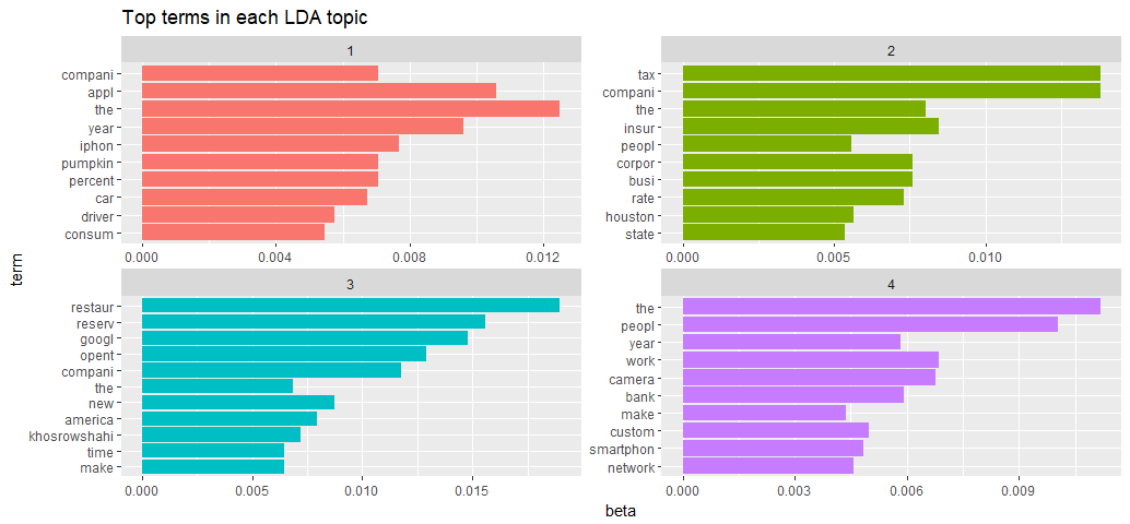
Let’s visualize to understand the 4 topics that were extracted from these 22 documents.
nytimes_top_terms <- nytimes_topics %>%
  group_by(topic) %>%
  top_n(10, beta) %>%
  ungroup() %>%
  arrange(topic, -beta)

nytimes_top_terms %>%
  mutate(term = reorder(term, beta)) %>%
  ggplot(aes(term, beta, fill = factor(topic))) +
  geom_col(show.legend = FALSE) +
  facet_wrap(~ topic, scales = "free") +
  coord_flip() + ggtitle('Top terms in each LDA topic')
The 4 topics generally look to describe:
- iPhone and car businesses
- Tax, insurance coroporates in Houson
- Restaurant reservation, Google, and Uber’s new CEO
- New technology and banking
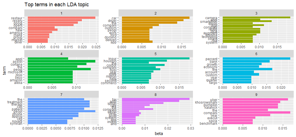
Let’s set k = 9, see how do our results change?
nytimes_lda <- LDA(dtm, k = 9, control = list(seed = 4321))
nytimes_topics <- tidy(nytimes_lda, matrix = "beta")

nytimes_top_terms <- nytimes_topics %>%
  group_by(topic) %>%
  top_n(10, beta) %>%
  ungroup() %>%
  arrange(topic, -beta)

nytimes_top_terms %>%
  mutate(term = reorder(term, beta)) %>%
  ggplot(aes(term, beta, fill = factor(topic))) +
  geom_col(show.legend = FALSE) +
  facet_wrap(~ topic, scales = "free") +
  coord_flip() + ggtitle('Top terms in each LDA topic')
From a quick view of the visualization it appears that the algorithm has done a decent job. The most common words in topic 9 include “uber” and “khosrowshahi”, which suggests it is about the new Uber CEO Dara Khosrowshahi. The most common words in topic 5 include “insurance”, “houston”, and “corporate”, suggesting that this topic represents insurance related matters after Houston’s Hurrican Harvey. One interesting observation is that the word “company” is common in 6 of the 9 topics.
For the interest of space, I fit a model with 9 topics to this dataset. I encourage you to try a range of different values of k (topic) to find the optimal number of topics, to see whether the model’s performance can be improved.
Document-topic probabilities
Besides estimating each topic as a mixture of words, topic modeling also models each document as a mixture of topics like so:
nytimes_lda_gamma <- tidy(nytimes_lda, matrix = "gamma")
nytimes_lda_gamma
### A tibble: 198 x 3
## document topic gamma
## <chr> <int> <dbl>
## 1 1 1 8.191867e-05
## 2 2 1 4.471408e-05
## 3 3 1 4.180694e-05
## 4 4 1 3.184344e-05
## 5 5 1 4.540474e-05
## 6 6 1 9.998000e-01
## 7 7 1 2.972724e-05
## 8 8 1 3.492409e-05
## 9 9 1 3.275588e-05
##10 10 1 3.918000e-05
### ... with 188 more rowsEach of these values (gamma) is an estimated proportion of words from that document that are generated from that topic. For example, the model estimates that about 0.008% of the words in document 1 were generated from topic 1. To confirm this result, we check what the most common words in document 1 were:
tidy(dtm) %>%
  filter(document == 1) %>%
  arrange(desc(count))
### A tibble: 177 x 3
## document term count
## <chr> <chr> <dbl>
## 1 1 driver 11
## 2 1 app 7
## 3 1 car 6
## 4 1 teenag 5
## 5 1 drive 4
## 6 1 parent 4
## 7 1 phone 4
## 8 1 compani 3
## 9 1 famili 3
##10 1 inform 3
### ... with 167 more rowsThis appears to be an article about teenagers’ driving. Topic 1 does not have driving related topics, this means that the algorithm was right not to place this document in topic 1.
The End
Topic modeling can provide a way to get from raw text to a deeper understanding of unstructured data. However, we need to examine the results carefully to check that they make sense.
So, try yourself, have fun, and start practicing those topic modeling skills!
