
As a runner myself, this dataset from Kaggle naturally got my attention. The dataset contains the name, age, gender, country, city and state (where available), times at 9 different stages of the race, expected time, finish time and pace, overall place, gender place and division place of 26630 finishers of 2016 Boston Marathon.
As alway, check the missing values, wrangle and clean up the data.
marathon <- read.csv('marathon_finishers_2016.csv', stringsAsFactors = F)
colnames(marathon) <- c('Bib', 'Name', 'Age', 'Gender', 'City', 'State', 'Country', 'Citizen', 'X', '5K', '10K', '15K', '20K', 'Half', '25K', '30K', '35K', '40K', 'Pace', 'Proj_Time', 'official_time', 'overall_place', 'Gender_place', 'Division_place')
drops <- c("State","Citizen", "X")
marathon <- marathon[ , !(names(marathon) %in% drops)]
marathon[!complete.cases(marathon),]
library(chron)
marathon$`5K` <- chron(times=marathon$`5K`)
marathon$`10K` <- chron(times = marathon$`10K`)
marathon$`15K` <- chron(times = marathon$`15K`)
marathon$`20K` <- chron(times = marathon$`20K`)
marathon$Half <- chron(times = marathon$Half)
marathon$`25K` <- chron(times = marathon$`25K`)
marathon$`35K` <- chron(times = marathon$`35K`)
marathon$`40K` <- chron(times = marathon$`40K`)
marathon$Pace <- chron(times = marathon$Pace)
marathon$Proj_Time <- chron(times = marathon$Proj_Time)
marathon$official_time <- chron(times = marathon$official_time)
Who were the finishers?
by(marathon$Age, marathon$Gender, summary)##marathon$Gender: F
## Min. 1st Qu. Median Mean 3rd Qu. Max.
## 18.0 31.0 40.0 39.9 47.0 83.0
##---------------------------------------------------------------
##marathon$Gender: M
## Min. 1st Qu. Median Mean 3rd Qu. Max.
## 18.0 36.0 45.0 44.7 53.0 83.0The youngest finishers were 18 years old, and oldest were 83, this applies to both genders.
library(ggplot2)
library(ggthemes)
ggplot(aes(x = Age, fill = Gender), data = marathon) +
  geom_histogram(position = position_dodge()) +
  scale_x_continuous(breaks = round(seq(min(marathon$Age), max(marathon$Age),
                                        by = 5),10)) +
  theme_economist() +
  ggtitle('Finishers by age and gender')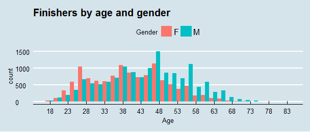
The number of female finishers is larger than male for younger runners, but this trend is reversed for older runners, and seems 48 is a good age to run for both male and female.
ggplot(aes(x=Gender, y=Age, fill=Gender), data = marathon) +
  geom_boxplot() +
  theme_economist() +
  ggtitle('Finishers Boxplot by Age and Gender')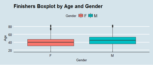
Female finishers are younger than male finishers in first quartile, median and third quartile.
marathon$age_group <- cut(marathon$Age, breaks=c(17,25,40,83), labels=c("18-25","26-40","41-83"))
library(dplyr)
gender_age_group <- group_by(marathon, Gender, age_group)
marathon_age_gender <- dplyr::summarise(gender_age_group, count = n(),
                                       average_time = mean(official_time))
marathon_age_gender$average_time <- 60 * 24 * as.numeric(times(marathon_age_gender$average_time))
ggplot(aes(x = Gender, y = count, fill = age_group), data = marathon_age_gender) +
  geom_bar(stat = 'identity', position = position_dodge()) +
  geom_text(stat='identity', aes(label = count),
            data = marathon_age_gender, position = position_dodge(width = 1)) +
  ggtitle('Total Finishers by Age and Gender')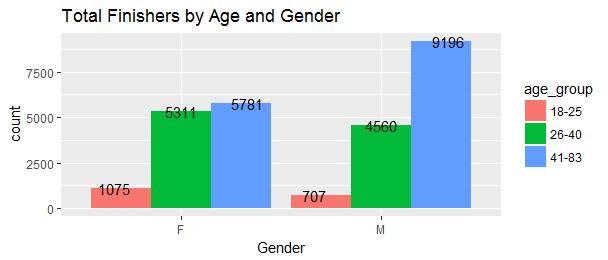
The split between men and women was 54% (14,463 runners) to 46% (12,167 runners), respectively. And over half (56%) of the finishers were older than 40. There were 9196 male age over 40 compared to just 5263 under 40. The picture looks different for female, there were 5781 female age over 40 compared to 6375 under 40.
ggplot(aes(x = Gender, y = average_time, fill=age_group), data=marathon_age_gender) + geom_bar(stat = 'identity', position = position_dodge()) +
  geom_text(stat='identity', aes(label = round(average_time)),
            data = marathon_age_gender, position = position_dodge(width=1)) +
  ylab('Average Finish Time (mins)') +
  ggtitle('Finish Time by Age and Gender')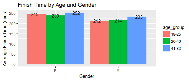
The average finish time difference based on age is not significant. 26-40 years old female had the best time in female group. There was almost no differnce on average finish time between 18 and 40 years old in male group.
Age matters
group_mean <- group_by(marathon, Age, Gender)
marathon_mean <- dplyr::summarise(group_mean, count = n(),
                                  mean = mean(official_time))

marathon_mean$mean <- 60 * 24 * as.numeric(times(marathon_mean$mean))
ggplot(aes(x = Age, y=mean, color=Gender), data = marathon_mean) +
  geom_point() + geom_line() +
  ylab('Average Finish Time(mins)') +
  ggtitle('Finish Time Trend by Age and Gender')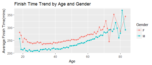
We can see young runners run faster as they mature. On average, there best time is at around 30 years old, after that, their finish time slowly increase. Of course there were outliers, several women age between 70 and 74 were faster than 60 years old men on average. There were men age between 75 and 79 finished within 4 hours.
Elite and the rest of us
According to Mercedes Marathon, to qualify for elite runners, the PR finishing time must be at least 2:35(155 mins) for men and 3:05(185 mins) for women. It makes sense to separate them from the rest of us.
marathon$official_time <- 60 * 24 * as.numeric(times(marathon$official_time))

marathon_m <- marathon[marathon$Gender == 'M',]
marathon_f <- marathon[marathon$Gender == 'F',]
marathon_elite_m <- marathon_m[marathon_m$official_time <= 155,]
marathon_elite_f <- marathon_f[marathon_f$official_time <= 185,]
marathon_normal_m <- marathon_m[marathon_m$official_time > 155,]
marathon_normal_f <- marathon_f[marathon_f$official_time > 185,]
marathon_elite <- rbind(marathon_elite_m, marathon_elite_f)
marathon_normal <- rbind(marathon_normal_m, marathon_normal_f)
ggplot(aes(x = official_time, color = Gender), data = marathon_elite) +
  geom_density() +
  xlab('Finish Time(mins)') +
  ggtitle('Elite Runners Finish Time')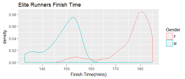
2016 Boston Marathon male and female winners were Lemi Berhanu Hayle and Atsede Baysa, crossed the line in 2:12:45 and 2:29:19, respectively. Most of the elite male runners crossed the finish line shortly after the 150-minute mark, and a great propotion of elite female runners crossed the finish line around the 180-minute mark.
by(marathon_normal$official_time, marathon_normal$Gender, summary)
ggplot(aes(x = official_time, color = Gender), data = marathon_normal) +
  geom_density() +
  scale_x_continuous(breaks = seq(155, 630, 25)) +
  xlab('Finish Time(mins)') +
  ggtitle('Average Runners Finish Time')
##marathon_normal$Gender: F
## Min. 1st Qu. Median Mean 3rd Qu. Max.
## 185 220 237 247 265 630
##---------------------------------------------------------------
##marathon_normal$Gender: M
## Min. 1st Qu. Median Mean 3rd Qu. Max.
## 155 197 218 226 248 505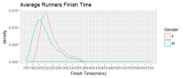
For the rest of us, the fastest male crossed finished line in 155 minutes (2:35) and 185 minutes (3:05) for female. The peak finish time for male was around 205 minutes (3:25) and for female was around 230 minutes (3:50).
When it comes to running, there is a gender gap between male and female, male, on average faster than female. And this gap is greater among the runners who finish last than among those who finish first.
Split
In running , a negative split is a racing strategy that involves completing the second half of a race faster than the first half. In contrast, positive split means running the second half slower than the first half. Even splits are where the two halves of the race are run in the same amount of time.
To add split in my analysis, I will need to do some calculation and add a column.
marathon$`5K` <- 60 * 24 * as.numeric(times(marathon$`5K`))
marathon$`10K` <- 60 * 24 * as.numeric(times(marathon$`10K`))
marathon$`15K` <- 60 * 24 * as.numeric(times(marathon$`15K`))
marathon$`20K` <- 60 * 24 * as.numeric(times(marathon$`20K`))
marathon$Half <- 60 * 24 * as.numeric(times(marathon$Half))
marathon$`25K` <- 60 * 24 * as.numeric(times(marathon$`25K`))
marathon$`30K` <- 60 * 24 * as.numeric(times(marathon$`30K`))
marathon$`35K` <- 60 * 24 * as.numeric(times(marathon$`35K`))
marathon$`40K` <- 60 * 24 * as.numeric(times(marathon$`40K`))
marathon$`5K`<- round(marathon$`5K`/5., 2)
marathon$`10K`<- round(marathon$`10K`/10., 2)
marathon$`15K` <- round(marathon$`15K`/15., 2)
marathon$`20K` <- round(marathon$`20K`/20., 2)
marathon$`25K` <- round(marathon$`25K`/25., 2)
marathon$Half <- round(marathon$Half/21., 2)
marathon$`30K` <- round(marathon$`30K`/30., 2)
marathon$`35K` <- round(marathon$`35K`/35., 2)
marathon$`40K` <- round(marathon$`40K`/40., 2)
marathon$secondhalf <- with(marathon, (`40K`+`35K`+`30K`+`25K`)/4)
marathon$firsthalf <- with(marathon, (`5K`+`10K`+`15K`+`20K`+Half)/5)
marathon$split <- with(marathon, secondhalf-firsthalf)
ggplot(aes(x = split, fill = Gender, color = Gender), data = marathon) +
  geom_density(position = 'stack') +
  xlab('Split') +
  ggtitle('Split Distribution') +
  theme_economist()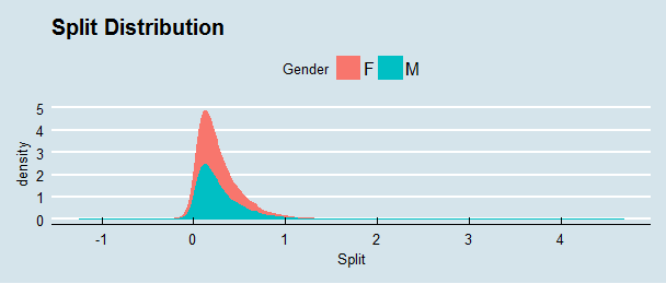
Majority of the runners ran a positive split. They ran second half slower than the first half, but not by much. There are a very small percent of runners ran a negative split. Are they elite runners?
marathon_elite$`5K` <- 60 * 24 * as.numeric(times(marathon_elite$`5K`))
marathon_elite$`10K` <- 60 * 24 * as.numeric(times(marathon_elite$`10K`))
marathon_elite$`15K` <- 60 * 24 * as.numeric(times(marathon_elite$`15K`))
marathon_elite$`20K` <- 60 * 24 * as.numeric(times(marathon_elite$`20K`))
marathon_elite$Half <- 60 * 24 * as.numeric(times(marathon_elite$Half))
marathon_elite$`25K` <- 60 * 24 * as.numeric(times(marathon_elite$`25K`))
marathon_elite$`30K` <- 60 * 24 * as.numeric(times(marathon_elite$`30K`))
marathon_elite$`35K` <- 60 * 24 * as.numeric(times(marathon_elite$`35K`))
marathon_elite$`40K` <- 60 * 24 * as.numeric(times(marathon_elite$`40K`))
marathon_elite$`5K`<- round(marathon_elite$`5K`/5., 2)
marathon_elite$`10K`<- round(marathon_elite$`10K`/10., 2)
marathon_elite$`15K` <- round(marathon_elite$`15K`/15., 2)
marathon_elite$`20K` <- round(marathon_elite$`20K`/20., 2)
marathon_elite$`25K` <- round(marathon_elite$`25K`/25., 2)
marathon_elite$Half <- round(marathon_elite$Half/21., 2)
marathon_elite$`30K` <- round(marathon_elite$`30K`/30., 2)
marathon_elite$`35K` <- round(marathon_elite$`35K`/35., 2)
marathon_elite$`40K` <- round(marathon_elite$`40K`/40., 2)
marathon_elite$secondhalf <- with(marathon_elite, (`40K`+`35K`+`30K`+`25K`)/4)
marathon_elite$firsthalf <- with(marathon_elite, (`5K`+`10K`+`15K`+`20K`+Half)/5)
marathon_elite$split <- with(marathon_elite, secondhalf-firsthalf)
ggplot(aes(x = split, fill = Gender, color = Gender), data = marathon_elite) +
  geom_density(position = 'stack') +
  xlab('Split') +
  ggtitle('Elite Runners Split Distribution') +
  theme_economist()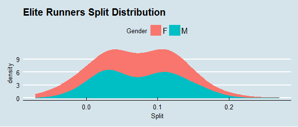
Indeed, there seems more negative split runners in the elite group, and even they run positive split, the difference is very very small(0 to 0.2 vs. non-elite runners’ 0 to 1), this indicates that they were able to maintain a very steady pace.
ggplot(aes(x = official_time, y = split, color = Gender), data = marathon) +
  geom_point(alpha=1/5) +
  geom_smooth(method='loess') +
  scale_color_brewer(type = "qual", palette = "Set1") +
  xlab('Finish Time (mins)') +
  ggtitle('Split and Finish Time') +
  theme_economist()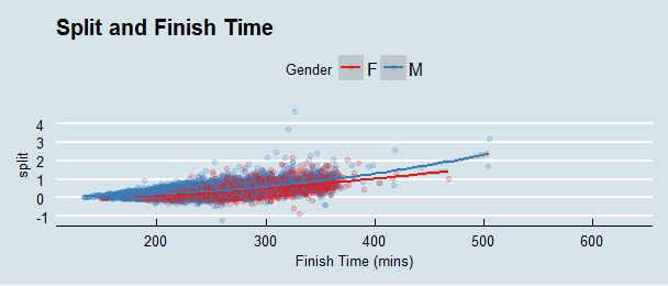
The general trend shows a moderate correlation between split and finish time, while a more positive split a runner runs, the more time he (or she) will need to finish.
Something else to consider
Because this is Boston, Up until about the 25K, most of the race is downhill. when reaching what they call “The Newton Hill” that end at about the 33.7K at the top of the so called “Heartbreak hill”. This hill is a test for many runners. Probably this is one of reasons why running a negative split is so hard.
The end
Boston Marathon 2017 is only less than three weeks away. If you run Boston this year, I hope this article can help put your race in context. Enjoy your race day!
Source code that create this post can be found here. I am happy to hear any feedback and questions.