
The data was extracted from 1994 Census bureau database. However, I downloaded from Kaggle at UCI Machine Learning Repository. The prediction task is to determine whether a person makes over $50K a year.
The data contains 32561 observations (people) and 15 variables. A high level summary of the data is below.
income <- read.csv('adult.csv', na.strings = c('','?'))
str(income)
##'data.frame': 32561 obs. of 15 variables:
## $ age : int 90 82 66 54 41 34 38 74 68 41 ...
## $ workclass : Factor w/ 8 levels "Federal-gov",..: NA 4 NA 4 4 4 4 7 1 4 ##...
## $ fnlwgt : int 77053 132870 186061 140359 264663 216864 150601 88638 ##422013 70037 ...
## $ education : Factor w/ 16 levels "10th","11th",..: 12 12 16 6 16 12 1 11 ##12 16 ...
## $ education.num : int 9 9 10 4 10 9 6 16 9 10 ...
## $ marital.status: Factor w/ 7 levels "Divorced","Married-AF-spouse",..: 7 7 7 ##1 6 1 6 5 1 5 ...
## $ occupation : Factor w/ 14 levels "Adm-clerical",..: NA 4 NA 7 10 8 1 10 ##10 3 ...
## $ relationship : Factor w/ 6 levels "Husband","Not-in-family",..: 2 2 5 5 4 ##5 5 3 2 5 ...
## $ race : Factor w/ 5 levels "Amer-Indian-Eskimo",..: 5 5 3 5 5 5 5 5 ##5 5 ...
## $ sex : Factor w/ 2 levels "Female","Male": 1 1 1 1 1 1 2 1 1 2 ...
## $ capital.gain : int 0 0 0 0 0 0 0 0 0 0 ...
## $ capital.loss : int 4356 4356 4356 3900 3900 3770 3770 3683 3683 3004 ...
## $ hours.per.week: int 40 18 40 40 40 45 40 20 40 60 ...
## $ native.country: Factor w/ 41 levels "Cambodia","Canada",..: 39 39 39 39 39 ##39 39 39 39 NA ...
## $ income : Factor w/ 2 levels "<=50K",">50K": 1 1 1 1 1 1 1 2 1 2 ...Statistics summary after changing missing values to ‘NA’.
summary(income)## age workclass fnlwgt education
## Min. :17.00 Private :22696 Min. : 12285 HS-grad :10501
## 1st Qu.:28.00 Self-emp-not-inc: 2541 1st Qu.: 117827 Some-college: 7291
## Median :37.00 Local-gov : 2093 Median : 178356 Bachelors : 5355
## Mean :38.58 State-gov : 1298 Mean : 189778 Masters : 1723
## 3rd Qu.:48.00 Self-emp-inc : 1116 3rd Qu.: 237051 Assoc-voc : 1382
## Max. :90.00 (Other) : 981 Max. :1484705 11th : 1175 ## NA's : 1836 (Other) : 5134
## education.num marital.status occupation
## Min. : 1.00 Divorced : 4443 Prof-specialty : 4140
## 1st Qu.: 9.00 Married-AF-spouse : 23 Craft-repair : 4099
## Median :10.00 Married-civ-spouse :14976 Exec-managerial: 4066
## Mean :10.08 Married-spouse-absent: 418 Adm-clerical : 3770
## 3rd Qu.:12.00 Never-married :10683 Sales : 3650
## Max. :16.00 Separated : 1025 (Other) :10993
## Widowed : 993 NA's : 1843
## relationship race sex capital.gain
## Husband :13193 Amer-Indian-Eskimo: 311 Female:10771 Min. : 0
## Not-in-family :8305 Asian-Pac-Islander: 1039 Male :21790 1st Qu.: 0
## Other-relative:981 Black : 3124 Median : 0
## Own-child : 5068 Other : 271 Mean : 1078
## Unmarried : 3446 White :27816 3rd Qu.: 0
## Wife : 1568 Max. :99999
## ## capital.loss hours.per.week native.country income
## Min. : 0.0 Min. : 1.00 United-States:29170 <=50K:24720
## 1st Qu.: 0.0 1st Qu.:40.00 Mexico : 643 >50K : 7841
## Median : 0.0 Median :40.00 Philippines : 198
## Mean : 87.3 Mean :40.44 Germany : 137
## 3rd Qu.: 0.0 3rd Qu.:45.00 Canada : 121
## Max. :4356.0 Max. :99.00 (Other) : 1709
## NA's : 583 Data Cleaning Process
Check for ‘NA’ values and look how many unique values there are for each variable.
sapply(income,function(x) sum(is.na(x)))## age workclass fnlwgt education education.num
## 0 1836 0 0 0
##marital.status occupation relationship race sex
## 0 1843 0 0 0
## capital.gain capital.loss hours.per.week native.country income
## 0 0 0 583 0 sapply(income, function(x) length(unique(x)))## age workclass fnlwgt education education.num
## 73 9 21648 16 16
##marital.status occupation relationship race sex
## 7 15 6 5 2
## capital.gain capital.loss hours.per.week native.country income
## 119 92 94 42 2 library(Amelia)
missmap(income, main = "Missing values vs observed")
table (complete.cases (income))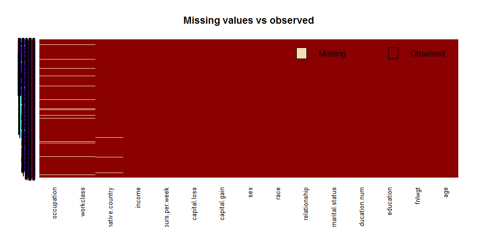
##FALSE  TRUE
## 2399 30162
Approximate 7%(2399/32561) of the total data has missing value. They are mainly in variables ‘occupation’, ‘workclass’ and ‘native country’. I decided to remove those missing values because I don’t think its a good idea to replace categorical values by imputing.
income <- income[complete.cases(income),]Explore Numeric Variables With Income Levels
library(ggplot2)
library(gridExtra)
p1 <- ggplot(aes(x=income, y=age), data = income) + geom_boxplot() +
  ggtitle('Age vs. Income Level')
p2 <- ggplot(aes(x=income, y=education.num), data = income) + geom_boxplot() +
  ggtitle('Years of Education vs. Income Level')
p3 <- ggplot(aes(x=income, y=hours.per.week), data = income) + geom_boxplot() +
  ggtitle('Hours Per Week vs. Income Level')
p4 <- ggplot(aes(x=income, y=capital.gain), data=income) + geom_boxplot() +
  ggtitle('Capital Gain vs. Income Level')
p5 <- ggplot(aes(x=income, y=capital.loss), data=income) + geom_boxplot() +
  ggtitle('Capital Loss vs. Income Level')
p6 <- ggplot(aes(x=income, y=fnlwgt), data=income) + geom_boxplot() +
  ggtitle('Final Weight vs. Income Level')
grid.arrange(p1, p2, p3, p4, p5, p6, ncol=3)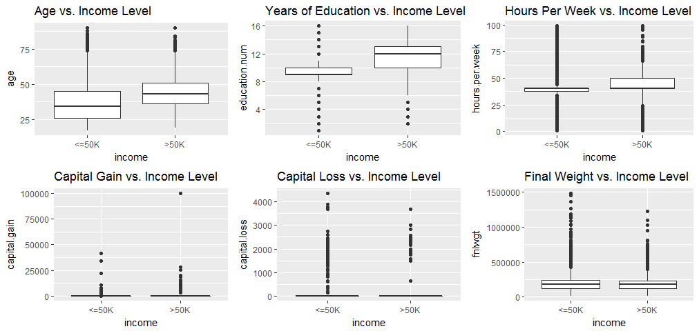
“Age”, “Years of education” and “hours per week” all show significant variations with income level. Therefore, they will be kept for the regression analysis. “Final Weight” does not show any variation with income level, therefore, it will be excluded from the analysis. Its hard to see whether “Capital gain” and “Capital loss” have variation with Income level from the above plot, so I will keep them for now.
income$fnlwgt <- NULLExplore Categorical Variables With Income Levels
library(dplyr)
by_workclass <- income %>% group_by(workclass, income) %>% summarise(n=n())
by_education <- income %>% group_by(education, income) %>% summarise(n=n())
by_education$education <- ordered(by_education$education,
                                   levels = c('Preschool', '1st-4th', '5th-6th', '7th-8th', '9th', '10th', '11th', '12th', 'HS-grad', 'Prof-school', 'Assoc-acdm', 'Assoc-voc', 'Some-college', 'Bachelors', 'Masters', 'Doctorate'))
by_marital <- income %>% group_by(marital.status, income) %>% summarise(n=n())
by_occupation <- income %>% group_by(occupation, income) %>% summarise(n=n())
by_relationship <- income %>% group_by(relationship, income) %>% summarise(n=n())
by_race <- income %>% group_by(race, income) %>% summarise(n=n())
by_sex <- income %>% group_by(sex, income) %>% summarise(n=n())
by_country <- income %>% group_by(native.country, income) %>% summarise(n=n())

p7 <- ggplot(aes(x=workclass, y=n, fill=income), data=by_workclass) + geom_bar(stat = 'identity', position = position_dodge()) + ggtitle('Workclass with Income Level') + theme(axis.text.x = element_text(angle = 45, hjust = 1))
p8 <- ggplot(aes(x=education, y=n, fill=income), data=by_education) + geom_bar(stat = 'identity', position = position_dodge()) + ggtitle('Education vs. Income Level') + coord_flip()
p9 <- ggplot(aes(x=marital.status, y=n, fill=income), data=by_marital) + geom_bar(stat = 'identity', position=position_dodge()) + ggtitle('Marital Status vs. Income Level') + theme(axis.text.x = element_text(angle = 45, hjust = 1))
p10 <- ggplot(aes(x=occupation, y=n, fill=income), data=by_occupation) + geom_bar(stat = 'identity', position=position_dodge()) + ggtitle('Occupation vs. Income Level') + coord_flip()
p11 <- ggplot(aes(x=relationship, y=n, fill=income), data=by_relationship) + geom_bar(stat = 'identity', position=position_dodge()) + ggtitle('Relationship vs. Income Level') + coord_flip()
p12 <- ggplot(aes(x=race, y=n, fill=income), data=by_race) + geom_bar(stat = 'identity', position = position_dodge()) + ggtitle('Race vs. Income Level') + coord_flip()
p13 <- ggplot(aes(x=sex, y=n, fill=income), data=by_sex) + geom_bar(stat = 'identity', position = position_dodge()) + ggtitle('Sex vs. Income Level')
p14 <- ggplot(aes(x=native.country, y=n, fill=income), data=by_country) + geom_bar(stat = 'identity', position = position_dodge()) + ggtitle('Native Country vs. Income Level') + coord_flip()
grid.arrange(p7, p8, p9, p10, ncol=2)
grid.arrange(p11, p12, p13, p14, ncol=2)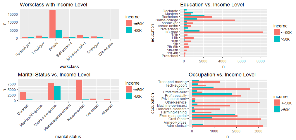
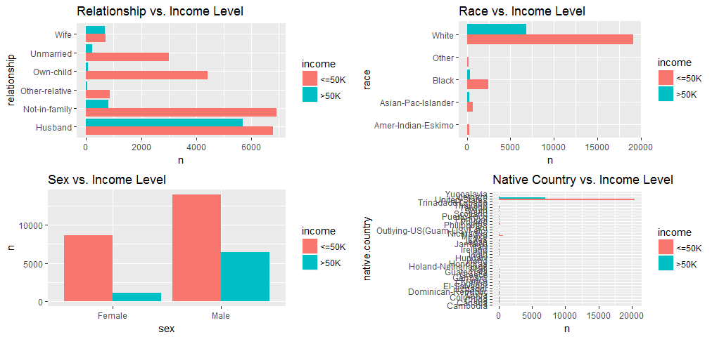
Most of the data was collected from the United States, so variable “native country” does not have effect on my analysis, I will exclude it from regression model. And all the other categorial variables seem to have reasonable variation, so will be kept.
income$native.country <- NULLincome$income = as.factor(ifelse(income$income==income$income[1],0,1))Convert income level to 0’s and 1’s,”<=50K” will be 0 and “>50K”” will be 1(binary outcome).
Model Fitting
split the data into two chunks: training and testing set.
train <- income[1:24000,]
test <- income[24001:30162,]
Fit the model
model <-glm(income ~.,family=binomial(link='logit'),data=train)
summary(model)
##Call:
##glm(formula = income ~ ., family = binomial(link = "logit"),
## data = train)
##Deviance Residuals:
## Min 1Q Median 3Q Max
##-5.1023 -0.5221 -0.1872 0.0581 3.3415
##Coefficients: (1 not defined because of singularities)
## Estimate Std. Error z value Pr(>|z|)
##(Intercept) -6.946e+00 4.711e-01 -14.743 < 2e-16 ***
##age 2.436e-02 1.888e-03 12.899 < 2e-16 ***
##workclassLocal-gov -6.826e-01 1.259e-01 -5.420 5.97e-08 ***
##workclassPrivate -4.959e-01 1.049e-01 -4.727 2.28e-06 ***
##workclassSelf-emp-inc -3.309e-01 1.383e-01 -2.392 0.016734 *
##workclassSelf-emp-not-inc -1.004e+00 1.228e-01 -8.181 2.82e-16 ***
##workclassState-gov -7.998e-01 1.401e-01 -5.708 1.15e-08 ***
##workclassWithout-pay -1.306e+01 2.386e+02 -0.055 0.956366
##education11th -7.654e-03 2.285e-01 -0.034 0.973272
##education12th 2.253e-01 3.101e-01 0.727 0.467456
##education1st-4th -6.456e-01 5.343e-01 -1.208 0.226955
##education5th-6th -7.638e-01 3.970e-01 -1.924 0.054348 .
##education7th-8th -7.297e-01 2.656e-01 -2.748 0.006003 **
##education9th -6.099e-01 3.093e-01 -1.972 0.048662 *
##educationAssoc-acdm 1.165e+00 1.941e-01 6.003 1.94e-09 ***
##educationAssoc-voc 1.088e+00 1.863e-01 5.840 5.23e-09 ***
##educationBachelors 1.784e+00 1.721e-01 10.366 < 2e-16 ***
##educationDoctorate 2.773e+00 2.433e-01 11.397 < 2e-16 ***
##educationHS-grad 6.298e-01 1.671e-01 3.769 0.000164 ***
##educationMasters 2.116e+00 1.851e-01 11.433 < 2e-16 ***
##educationPreschool -2.026e+01 1.422e+02 -0.142 0.886719
##educationProf-school 2.641e+00 2.266e-01 11.654 < 2e-16 ***
##educationSome-college 9.415e-01 1.698e-01 5.544 2.96e-08 ***
##education.num NA NA NA NA
##marital.statusMarried-AF-spouse 3.113e+00 6.846e-01 4.548 5.43e-06 ***
##marital.statusMarried-civ-spouse 2.071e+00 3.025e-01 6.846 7.57e-12 ***
##marital.statusMarried-spouse-absent -9.842e-02 2.684e-01 -0.367 0.713876
##marital.statusNever-married -4.215e-01 9.933e-02 -4.243 2.20e-05 ***
##marital.statusSeparated 4.981e-02 1.795e-01 0.277 0.781443
##marital.statusWidowed 1.641e-01 1.811e-01 0.906 0.364857
##occupationArmed-Forces -1.030e+00 1.519e+00 -0.678 0.497620
##occupationCraft-repair 1.312e-01 8.996e-02 1.458 0.144763
##occupationExec-managerial 8.642e-01 8.719e-02 9.912 < 2e-16 ***
##occupationFarming-fishing -9.219e-01 1.556e-01 -5.927 3.09e-09 ***
##occupationHandlers-cleaners -6.340e-01 1.624e-01 -3.903 9.50e-05 ***
##occupationMachine-op-inspct -2.581e-01 1.148e-01 -2.248 0.024571 *
##occupationOther-service -7.466e-01 1.302e-01 -5.735 9.74e-09 ***
##occupationPriv-house-serv -4.065e+00 1.761e+00 -2.309 0.020966 *
##occupationProf-specialty 5.969e-01 9.185e-02 6.499 8.11e-11 ***
##occupationProtective-serv 6.089e-01 1.401e-01 4.345 1.39e-05 ***
##occupationSales 3.265e-01 9.278e-02 3.519 0.000434 ***
##occupationTech-support 7.090e-01 1.247e-01 5.684 1.31e-08 ***
##occupationTransport-moving 6.729e-03 1.104e-01 0.061 0.951385
##relationshipNot-in-family 3.903e-01 2.989e-01 1.306 0.191598
##relationshipOther-relative -4.501e-01 2.736e-01 -1.645 0.100029
##relationshipOwn-child -7.227e-01 2.971e-01 -2.433 0.014990 *
##relationshipUnmarried 2.333e-01 3.171e-01 0.736 0.461827
##relationshipWife 1.344e+00 1.176e-01 11.424 < 2e-16 ***
##raceAsian-Pac-Islander 2.932e-01 2.811e-01 1.043 0.296968
##raceBlack 4.212e-01 2.667e-01 1.579 0.114232
##raceOther -5.576e-01 4.370e-01 -1.276 0.201988
##raceWhite 4.978e-01 2.549e-01 1.953 0.050844 .
##sexMale 8.690e-01 8.981e-02 9.677 < 2e-16 ***
##capital.gain 3.239e-04 1.083e-05 29.899 < 2e-16 ***
##capital.loss 6.432e-04 3.870e-05 16.622 < 2e-16 ***
##hours.per.week 2.840e-02 1.912e-03 14.854 < 2e-16 ***
##---
##Signif. codes: 0 ‘***’ 0.001 ‘**’ 0.01 ‘*’ 0.05 ‘.’ 0.1 ‘ ’ 1
##(Dispersion parameter for binomial family taken to be 1)
## Null deviance: 27607 on 23999 degrees of freedom
##Residual deviance: 15626 on 23945 degrees of freedom
##AIC: 15736
##Number of Fisher Scoring iterations: 13Interpreting the results of the logistic regression model:
- “Age”, “Hours per week”, “sex”, “capital gain” and “capital loss” are the most statistically significant variables. Their lowest p-values suggesting a strong association with the probability of wage>50K from the data.
- “Workclass”, “education”, “marital status”, “occupation” and “relationship” are all across the table. so cannot be eliminated from the model.
- “Race” category is not statistically significant and can be eliminated from the model.
Run the anova() function on the model to analyze the table of deviance.
anova(model, test="Chisq")##Analysis of Deviance Table
##Model: binomial, link: logit
##Response: income
##Terms added sequentially (first to last)
## Df Deviance Resid. Df Resid. Dev Pr(>Chi)
##NULL 23999 27607
##age 1 1390.0 23998 26217 < 2.2e-16 ***
##workclass 6 357.4 23992 25859 < 2.2e-16 ***
##education 15 3009.1 23977 22850 < 2.2e-16 ***
##education.num 0 0.0 23977 22850
##marital.status 6 4121.0 23971 18729 < 2.2e-16 ***
##occupation 13 634.8 23958 18094 < 2.2e-16 ***
##relationship 5 167.8 23953 17927 < 2.2e-16 ***
##race 4 19.9 23949 17907 0.0005157 ***
##sex 1 136.3 23948 17770 < 2.2e-16 ***
##capital.gain 1 1625.5 23947 16145 < 2.2e-16 ***
##capital.loss 1 293.2 23946 15852 < 2.2e-16 ***
##hours.per.week 1 225.6 23945 15626 < 2.2e-16 ***
##---
##Signif. codes: 0 ‘***’ 0.001 ‘**’ 0.01 ‘*’ 0.05 ‘.’ 0.1 ‘ ’ 1The difference between the null deviance and the residual deviance indicates how the model is doing against the null model. The bigger difference, the better. From the above table we can see the drop in deviance when adding each variable one at a time. Adding age, workclass, education, marital status, occupation, relationship, race, sex, capital gain, capital loss and hours per week significantly reduces the residual deviance. education.num seem to have no effect.
Apply model to the test set
fitted.results <- predict(model,newdata=test,type='response')
fitted.results <- ifelse(fitted.results > 0.5,1,0)
misClasificError <- mean(fitted.results != test$income)
print(paste('Accuracy',1-misClasificError))
##[1] "Accuracy 0.844368711457319"The 0.84 accuracy on the test set is a very encouraging result.
At last, plot the ROC curve and calculate the AUC (area under the curve). The closer AUC for a model comes to 1, the better predictive ability.
library(ROCR)
p <- predict(model, newdata=test, type="response")
pr <- prediction(p, test$income)
prf <- performance(pr, measure = "tpr", x.measure = "fpr")
plot(prf)
auc <- performance(pr, measure = "auc")
auc <- auc@y.values[[1]]
auc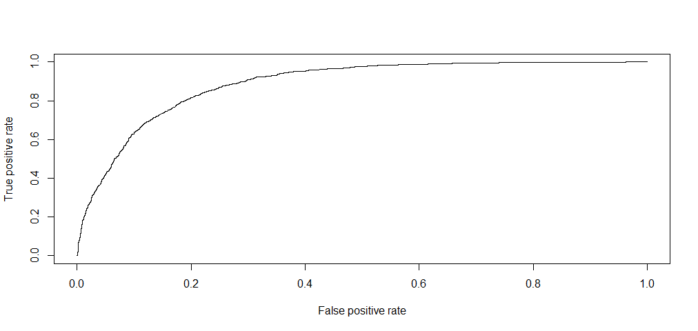
##[1] 0.8868877The area under the curve corresponds the AUC.
As a last step, as I have just learned, use the effects package to compute and plot all variables.
library(effects)
plot(allEffects(model))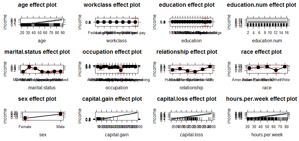
The End
I have been very cautious on removing variables because I don’t want to compromise the data as I may end up removing valid information. As a result, I may have kept variables that I should have removed such as “education.num”.
Source code that created this post can be found here. I am happy to hear any feedback or questions.
Reference: r-bloggers