
Setup
Load packages
library(ggplot2)
library(dplyr)
library(statsr)
Load data
load("gss.rdata")Part 1: Data
Background
The General Social Survey (GSS) is a sociological survey used to collect information and keep a historical record of the concerns, experiences, attitudes, and practices of residents of the United States. GSS questions cover a diverse range of issues including national spending priorities, marijuana use, crime and punishment, race relations, quality of life, confidence in institutions, and sexual behavior. The dataset used for this project is an extract of the General Social Survey (GSS) Cumulative File 1972-2012. It consists of 57061 observations with 114 variables. Each variable corresponds to a specific question asked to the respondent.
Methodology
According to Wikipedia, The GSS survey is conducted face-to-face with an in-person interview by NORC at the University of Chicago. The target population is adults (18+) living in households in the United States. Respondents are random sampled from a mix of urban, suburban, and rural geographic areas. Participation in the study is strictly voluntary.
The scope of inference
The sample data should allow us to generalize to the population of interest. It is a survey of 57061 U.S adults aged 18 years or older. The survey is based on random sampling. However, there is no causation can be established as GSS is an observation study that can only establish correlation/association between variables. In addition, potential biases are associated with non-response because this is a voluntary in-person survey that takes approximately 90 minutes. Some potential respondents may choose not to participate.
Part 2: Research questions
Research Question 1: Do Americans distrust the media? That is, correlation between reading news and confidence in press.
According to Financial Times, Public trust in traditional media has fallen to an all-time low as people increasingly favour their friends and contacts on the internet as sources of news. This has prompted me to learn how frequency of reading news may impact a person’s confidence in press. Based on above question, the analysis will be based on the following variables:
- news - How often does respondent read newspaper.
- conpress - Confidence in press.
To reflect the most recent trends, I will only keep the data from year 2010 and removing all “NA”s.
gss_con <- gss[ which(gss$year >= 2010 & !is.na(gss$news) & !is.na(gss$conpress)), ]
gss_con <- gss_con %>% select(news, conpress)
dim(gss_con)
##[1] 1398 2Exploratory data analysis for Research Question 1
The data I will be using for this analysis has 1398 observations. Here is the summary and two-way table.
summary(gss_con)## news conpress
## Everyday :452 A Great Deal:129
## Few Times A Week :241 Only Some :612
## Once A Week :192 Hardly Any :657
## Less Than Once Wk:224
## Never :289 table(gss_con$news, gss_con$conpress)## A Great Deal Only Some Hardly Any
## Everyday 50 206 196
## Few Times A Week 18 111 112
## Once A Week 19 85 88
## Less Than Once Wk 18 97 109
## Never 24 113 152plot(table(gss_con$news, gss_con$conpress))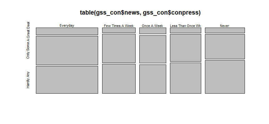
Mosaic plots provide a way to visualize contingency tables. If we compare the mosaic plot to the table of counts, the size of the boxes are related to the counts in the table. We can see that the number of respondents who read every day and only have some confidence in press are the highest, and the number of respondents who read few times a week and have great confidence in press are the lowest.
ggplot(aes(x=news), data=gss_con) + geom_bar(aes(fill=conpress), position = position_dodge()) + ggtitle('Frequency of Reading News vs. Confidence in Press')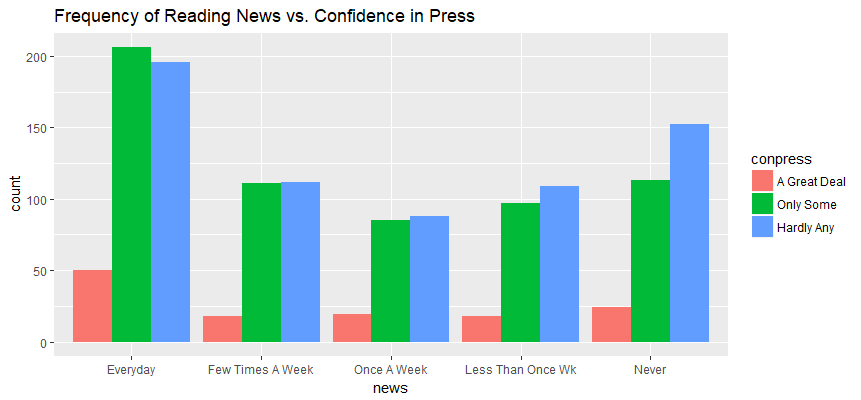
Observations:
- The number of respondents who have a great deal of confidence in press are consistently lowest across all groups of news readers.
- The number of respondents who hardly have any confidence in press are highest in three group of news readers - “Never”, “Less than Once Wk” and “Once A Week”.
Inference for Research Question 1
State hypothesis
Null Hypothesis: Frequency of reading news and confidence in press are independent. Frequency of reading news does not vary by confidence in press.
Alternative Hypothesis: Frequency of reading news and confidence in press are dependent. Frequency of reading news does vary by confidence in press.
Check conditions
- The survey respondents were random sampled, we can assume the independence.
- If sampling without replacement, n < 10% of population. The 1398 observations met this requirement.
- Each case only contribute to one cell in the table. Because the independence requirement has been met, we can check this as well.
- Each cell must have at least 5 expected cases. From below table, it is clear that it meets the requirement.
gss_con_table <- table(gss_con$news, gss_con$conpress)
Xsq <- chisq.test(gss_con_table)
Xsq$expected
## A Great Deal Only Some Hardly Any
## Everyday 41.70815 197.87124 212.42060
## Few Times A Week 22.23820 105.50215 113.25966
## Once A Week 17.71674 84.05150 90.23176
## Less Than Once Wk 20.66953 98.06009 105.27039
## Never 26.66738 126.51502 135.81760State method to be used and why and how
The method used here is Chi-Square Independence Test since we are quantifying how different the observed counts are from the expected counts and we are evaluating relationship between two categorical variables.
Perform inference
(Xsq <- chisq.test(gss_con_table))##Pearson's Chi-squared test
##data: gss_con_table
##X-squared = 8.6459, df = 8, p-value = 0.373The Chi-Squre statistic is 8.6459, degree of freedom is 8 and the associated P value is larger than the significance level of 0.05.
Interpret results
We failed to reject null hypothesis, the data does not provide convincing evidence that the frequency of reading news and confidence in press are associated.
Research Question 2: Does marital status have impact on financial satisfaction?
According to a report from The National Center for Biotechnology Information (NCBI), people who are financially satisfied tend to be more stable in their marriages. I am interested to find out whether satisfaction in financial situation is associated with marital status, by analyzing GSS data. I will be using the following variables for this analysis:
- marital - Marital status
- satfin - Satifaction with financial situation
I will remove “NA”s and keep all years data.
Exploratory data analysis for Research Question 2
gss_ma <- gss[ which(!is.na(gss$marital) & !is.na(gss$satfin)), ]
gss_ma <- gss_ma %>% select(marital, satfin)
dim(gss_ma)
##[1] 52441 2The data I will be using for this analysis have 52441 observations. Here is the summary and two-way table.
summary(gss_ma)
table(gss_ma$marital, gss_ma$satfin)
## marital satfin
## Married :28417 Satisfied :15341
## Widowed : 5171 More Or Less :23172
## Divorced : 6362 Not At All Sat:13928
## Separated : 1833
## Never Married:10658 ## Satisfied More Or Less Not At All Sat
## Married 9281 13002 6134
## Widowed 1925 2150 1096
## Divorced 1256 2660 2446
## Separated 253 736 844
## Never Married 2626 4624 3408plot(table(gss_ma$marital, gss_ma$satfin))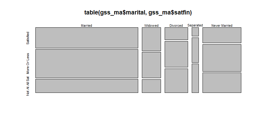
Interesting to see that the number of respondents who are “married” and “satisfied” are not the highest across all the groups. Seems people are hard to please.
ggplot(aes(x=marital), data=gss_ma) + geom_bar(aes(fill=satfin), position = position_dodge()) + ggtitle('Marital Status vs. Financial Satisfaction')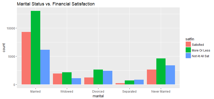
Observations:
- The number of respondents who are more or less satisfied with financial situation are the highest across all groups of marital status except “Separated” group.
- The number of respondents who are not at all satisfied with financial situation are lowest in “Married” and “Widowed” groups.
- The number of respondents who are satisfied with financial situation are lowest in “Never Married”, “Separated” and “Divorced” groups.
Inference for Research Question 2
State hypothesis
Null Hypothesis: Marital status and satisfaction with financial situation are independent. Satisfaction with financial situation does not vary by marital status.
Alternative Hypothesis: Marital status and satisfaction with financial situation are dependent. Satisfaction with financial situation does vary by marital status.
Check conditions
- The independence and sampling population (n < 10%) have been discussed earlier.
- Each cell must have at least 5 expected cases. From below table, it is clear that it meets the requirement
gss_ma_table <- table(gss_ma$marital, gss_ma$satfin)
Xsq1 <- chisq.test(gss_ma_table)
Xsq1$expected
## Satisfied More Or Less Not At All Sat
## Married 8313.0603 12556.5631 7547.3766
## Widowed 1512.7155 2284.8994 1373.3851
## Divorced 1861.1285 2811.1642 1689.7072
## Separated 536.2227 809.9441 486.8333
## Never Married 3117.8730 4709.4292 2830.6978State method to be used and why and how
Again, the method used here is Chi-Square Independence Test since we are quantifying how different the observed counts are from the expected counts and we are evaluating relationship between two categorical variables.
Perform inference
(Xsq1 <- chisq.test(gss_ma_table))##Pearson's Chi-squared test
##data: gss_ma_table
##X-squared = 1728.2, df = 8, p-value < 2.2e-16The Chi-Squre statistic is 1728.2, degree of freedom is 8 and the associated P value is almost 0.
Interpret results
With such a small P value, We reject null hypothesis in favor of alternative hypothesis and conclude that satisfaction with financial situation and marital status are dependent. The study is observational, so we can only establish association but not causation between these two variables.
Research Question 3: Income disparity among races
The existence of racial wage gap in America has been documented by many scholars and written about in many journals. Some research finds that the racial wage gap is focused in the private sector. How about U.S citizen in general? I am interested in drawing statistical inference using GSS data to compare family income between difference races. I will be using the following variables for this analysis:
- race: Race of respondent
- coninc: Total family income in constant dollars
Again, remove all “NA”s and keep data for all the years.
Exploratory data analysis for Research Question 3
gss_in <- gss[ which(!is.na(gss$race) & !is.na(gss$coninc)), ]
gss_in <- gss_in %>% select(race, coninc)
dim(gss_in)
##[1] 51232 2The data I will be using for this analysis has 51232 observations and 2 variables.
ggplot(aes(x=race, y=coninc), data=gss_in) + geom_boxplot() + ggtitle('Race vs. Family Income Boxplot')
by(gss_in$coninc, gss_in$race, summary)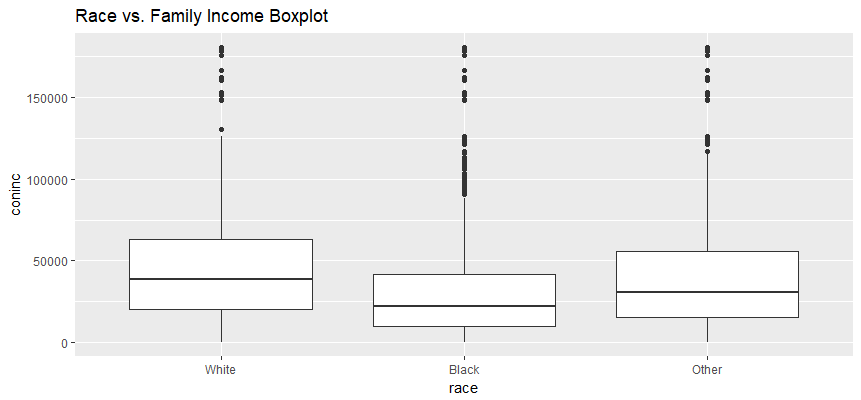
##gss_in$race: White
##   Min. 1st Qu.  Median    Mean 3rd Qu.    Max.
##    383   20129   38414   47007   62946  180386
##--------------------------------------------------------------
##gss_in$race: Black
##   Min. 1st Qu.  Median    Mean 3rd Qu.    Max.
##    383    9953   21959   30185   41523  180386
##--------------------------------------------------------------
##gss_in$race: Other
##   Min. 1st Qu.  Median    Mean 3rd Qu.    Max.
##    383   15572   30861   42415   56059  180386
Observations:
- The distribution of total family incomce for all race groups are right skewed.
- The White group has the highest total family income in first quartile, median, mean and 3rd quartile.
- The Black group has the least variability in total family income.
Inference for Research Question 3
State hypothesis
Null Hypothesis: The average total family income is the same across all the race groups.
Alternative Hypothesis: The average total family income differ between at least one pair of the race groups.
Check conditions
- The survey respondents were random sampled and the samples are less than 10% of population. So the condition of independence within group is met.
- We have three race groups and they are independent of each other.
- Distribution of response variable in each race group should be approximately normal. Unfortunatley, from below QQ plot, we can see all three groups have quite a bit divergence from normality in the upper tail.
qqnorm(gss_in$coninc[gss_in$race=='White'], main="White")
qqline(gss_in$coninc[gss_in$race=='White'])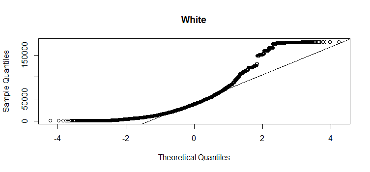
qqnorm(gss_in$coninc[gss_in$race=='Black'], main="Black")
qqline(gss_in$coninc[gss_in$race=='Black'])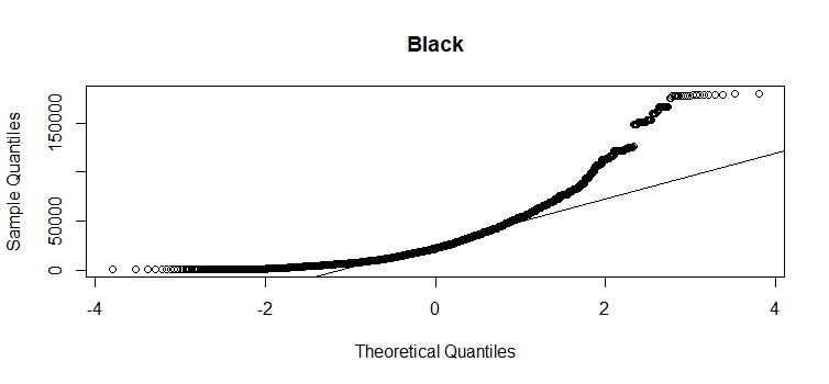
qqnorm(gss_in$coninc[gss_in$race=='Other'], main="Other")
qqline(gss_in$coninc[gss_in$race=='Other'])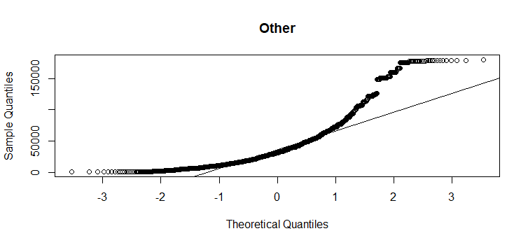
- Variability should be consistent across groups. From above boxplot, it seems that the variability is consistent across “White” and “Other” groups, but it is much lower for the “Black” group.
Although the assumptions of ANOVA did not meet, I will still go ahead to perform ANOVA but I have to be very careful in interpreting the results.
State method to be used and why and how
We compare average family income from more than two groups, - “White”, “Black” and “Other”. We want to know whether those three means are so far apart that the observed differences cannot all reasonably be attributed to sampling variability. So we use ANOVA.
mod <- lm(coninc ~ race, data = gss_in)
anova(mod)
##Analysis of Variance Table
##Response: coninc
## Df Sum Sq Mean Sq F value Pr(>F)
##race 2 1.6989e+12 8.4944e+11 675.08 < 2.2e-16 ***
##Residuals 51229 6.4461e+13 1.2583e+09
##---
##Signif. codes: 0 '***' 0.001 '**' 0.01 '*' 0.05 '.' 0.1 ' ' 1Interpret results
With such a small P value (almost 0), we reject the null hypothesis, we have sufficient evidence that at least one pair of race groups’ population average family income are different from each other. But we don’t know which pair of groups.
Since the results of ANOVA was significant, we are safe to continue with our pairwise comparisons to find out which pair of groups have difference income.
pairwise.t.test(gss_in$coninc, gss_in$race, p.adj ='bonferroni')##Pairwise comparisons using t tests with pooled SD
##data: gss_in$coninc and gss_in$race
## White Black
##Black < 2e-16 -
##Other 1.4e-09 < 2e-16
##P value adjustment method: bonferroni Using the Bonferroni adjustment, all group pairs, White-Black, White-Other, Black-Other comparisons are statistically significant. We are using a more stringent and conservative correction (Bonferroni adjustment) and we still got very small P values, therefore, we can reject the null hypothesis again.
Confidence Interval
As a last step, calculate confidence interval for one pairwise group difference - “White” and “Other”.
gss_in_w_o <- subset(gss_in, race== 'White' | race=='Other', select=c(race, coninc))
gss_in_w_o <- droplevels(gss_in_w_o)
inference(y = coninc, x = race, data = gss_in_w_o, statistic = "mean", type = "ci", conf_level = 0.95, method = "theoretical")
##Response variable: numerical, Explanatory variable: categorical (2 levels)
##n_White = 41824, y_bar_White = 47006.7433, s_White = 36405.4758
##n_Other = 2452, y_bar_Other = 42415.4274, s_Other = 38105.4353
##95% CI (White - Other): (3042.4667 , 6140.165)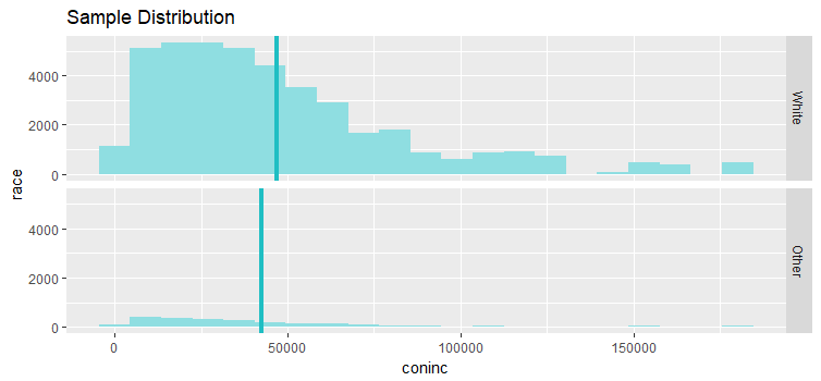
Conclusion
We are 95% confident that the average total family income of the “White” group was $3042 to $6140 higher than the “Other” group per year.
Here we performed ANOVA to assess whether a significant difference exists at all amongst the groups, whereas the pairwise comparisons were used to determine which group differences are statistically significant. Although our data have significant divergence from normality for all three race groups, ANOVA is considered a robust test against the normality assumption.
References:
Pearson’s Chi-squared test for count data