
There’s rightly been a lot of attention paid to text mining. Text mining is the data analysis of natural language works (articles, books, etc.), using text as a form of data, joined with the numeric analysis.
Two years ago, TheStreet claimed that Traders Are Using Text and Data Mining to Beat the Market. All this, and the sense of major things going on in the world, prompted me to see what I could find myself in the world of text mining.
library(tm.plugin.webmining)
library(purrr)
library(dplyr)
library(ggplot2)
library(ggthemes)
library(stringr)
library(tidyr)
library(tidytext)
Thus, I decided to analyze Google finance articles for the following American companies: Starbucks, Kraft, Wal-Mart and Mondelez.
company <- c("Starbucks", "Kraft", "Walmart", "Mondelez")
symbol <- c("SBUX", "KHC", "WMT", "MDLZ")
download_articles <- function(symbol) {
  WebCorpus(GoogleFinanceSource(paste0("NASDAQ:", symbol)))
}
stock_articles <- data_frame(company = company,
                             symbol = symbol) %>%
  mutate(corpus = map(symbol, download_articles))
Google Finance Articles
This allows me to retrieve the 20 most recent articles related to each stock.
stock_articles### A tibble: 4 × 3
## company symbol corpus
## <chr> <chr> <list>
##1 Starbucks SBUX <S3: WebCorpus>
##2 Kraft KHC <S3: WebCorpus>
##3 Walmart WMT <S3: WebCorpus>
##4 Mondelez MDLZ <S3: WebCorpus>Tokens
A token is a meaningful unit of text, most often a word, that we are interested in using for further analysis, and tokenization is the process of splitting text into tokens. I need to use “unnest_tokens” to break text into individual tokens and transform it to a tidy data, that is one-row-per-term-per-document:
tokens <- stock_articles %>%
  unnest(map(corpus, tidy)) %>%
  unnest_tokens(word, text) %>%
  select(company, datetimestamp, word, id, heading)
tokens
### A tibble: 59,572 × 5
## company datetimestamp word
## <chr> <dttm> <chr>
##1 Starbucks 2017-05-23 04:37:30 tesla
##2 Starbucks 2017-05-23 04:37:30 forum
##3 Starbucks 2017-05-23 04:37:30 summary
##4 Starbucks 2017-05-23 04:37:30 mobile
##5 Starbucks 2017-05-23 04:37:30 order
##6 Starbucks 2017-05-23 04:37:30 app
##7 Starbucks 2017-05-23 04:37:30 is
##8 Starbucks 2017-05-23 04:37:30 an
##9 Starbucks 2017-05-23 04:37:30 important
##10 Starbucks 2017-05-23 04:37:30 long
### ... with 59,562 more rows, and 2 more variables: id <chr>, heading <chr>tf_idf
article_tf_idf <- tokens %>%
  count(company, word) %>%
  filter(!str_detect(word, "\\d+")) %>%
  bind_tf_idf(word, company, n) %>%
  arrange(-tf_idf)
article_tf_idf
##Source: local data frame [9,966 x 6]
##Groups: company [4]
## company word n tf idf tf_idf
## <chr> <chr> <int> <dbl> <dbl> <dbl>
##1 Kraft heinz 128 0.014134276 1.3862944 0.019594267
##2 Starbucks starbucks 284 0.016820659 0.6931472 0.011659192
##3 Kraft khc 74 0.008171378 1.3862944 0.011327935
##4 Kraft kraft 139 0.015348940 0.6931472 0.010639074
##5 Walmart west 81 0.005955882 1.3862944 0.008256606
##6 Walmart environmental 78 0.005735294 1.3862944 0.007950806
##7 Walmart mountain 87 0.006397059 0.6931472 0.004434103
##8 Starbucks sbux 105 0.006218905 0.6931472 0.004310617
##9 Walmart virginia 36 0.002647059 1.3862944 0.003669603
##10 Walmart clarke 35 0.002573529 1.3862944 0.003567669
### ... with 9,956 more rowsHere we see all nouns, names that are important in these companies(articles). None of them occurred in all of the articles.
tf_idf, short for term frequency–inverse document frequency, is a numerical statistic that is intended to reflect how important a word is to a document in a collection or corpus.
Visualize these high tf-idf words.
plot_article <- article_tf_idf %>%
  arrange(desc(tf_idf)) %>%
  mutate(word = factor(word, levels = rev(unique(word))))
plot_article %>%
  top_n(10) %>%
  ggplot(aes(word, tf_idf, fill = company)) +
  geom_col() +
  labs(x = NULL, y = "tf-idf") +
  coord_flip() + theme_minimal() + ggtitle('Highest tf_idf Words for Each Company')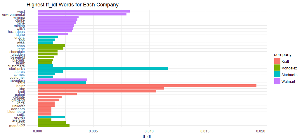
Visualize the top terms for each company individually.
plot_article %>%
  group_by(company) %>%
  top_n(10) %>%
  ungroup %>%
  ggplot(aes(word, tf_idf, fill = company)) +
  geom_col(show.legend = FALSE) +
  labs(x = NULL, y = "tf-idf") +
  facet_wrap(~company, ncol = 2, scales = "free") +
  coord_flip() + theme_minimal()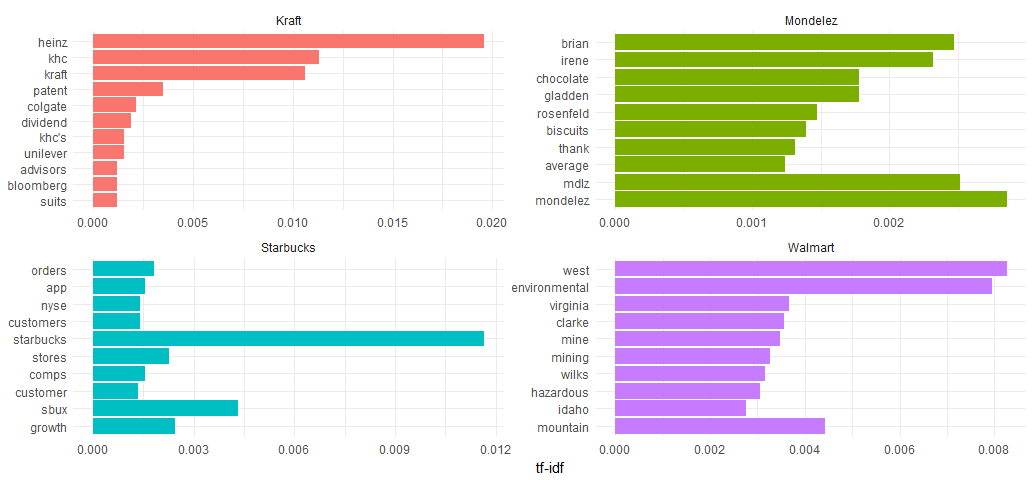
As we have expected, the company names, stock symbols, some of companies’ products and executives are usually included, as well as companies’ latest movements such as Wal-Mart’s climate pledges.
Sentiment
To see whether the finance news coverage is positive or negative for these four companies, I opted to use AFINN lexicons which provides a positivity score for each word, from -5 (most negative) to 5 (most positive) to do a simple sentiment analysis.
tokens %>%
  anti_join(stop_words, by = "word") %>%
  count(word, id, sort = TRUE) %>%
  inner_join(get_sentiments("afinn"), by = "word") %>%
  group_by(word) %>%
  summarize(contribution = sum(n * score)) %>%
  top_n(15, abs(contribution)) %>%
  mutate(word = reorder(word, contribution)) %>%
  ggplot(aes(word, contribution)) +
  geom_col() +
  coord_flip() +
  ggtitle('Frequency of Words AFINN Score') + theme_minimal()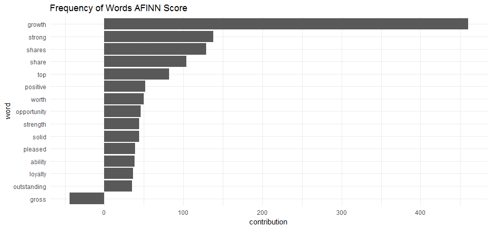
If I am right then I can use the sentiment analysis to help make decision on my investment. But am I right?
The word “gross” is considered negative by AFINN lexicons, but it means “gross margin” in the context of finance articles. The word “share” and “shares” are neither positive nor negative in finance articles, but here AFINN lexicons count them as positive.
“tidytext” includes another sentiment lexicon - “loughran”, which was developed based on analyses of financial reports, and intentionally avoids words like “share” and “gross” that may not have a positive or negative meaning in a financial context.
The Loughran dictionary divides words into six sentiments: “positive”, “negative”, “litigious”, “uncertainty”, “constraining”, and “superfluous”.
library(tidytext)
tokens %>%
  count(word) %>%
  inner_join(get_sentiments("loughran"), by = "word") %>%
  group_by(sentiment) %>%
  top_n(5, n) %>%
  ungroup() %>%
  mutate(word = reorder(word, n)) %>%
  ggplot(aes(word, n)) +
  geom_col() +
  coord_flip() +
  facet_wrap(~ sentiment, scales = "free") +
  ggtitle("Frequency of This Word in Google Finance Articles") + theme_minimal()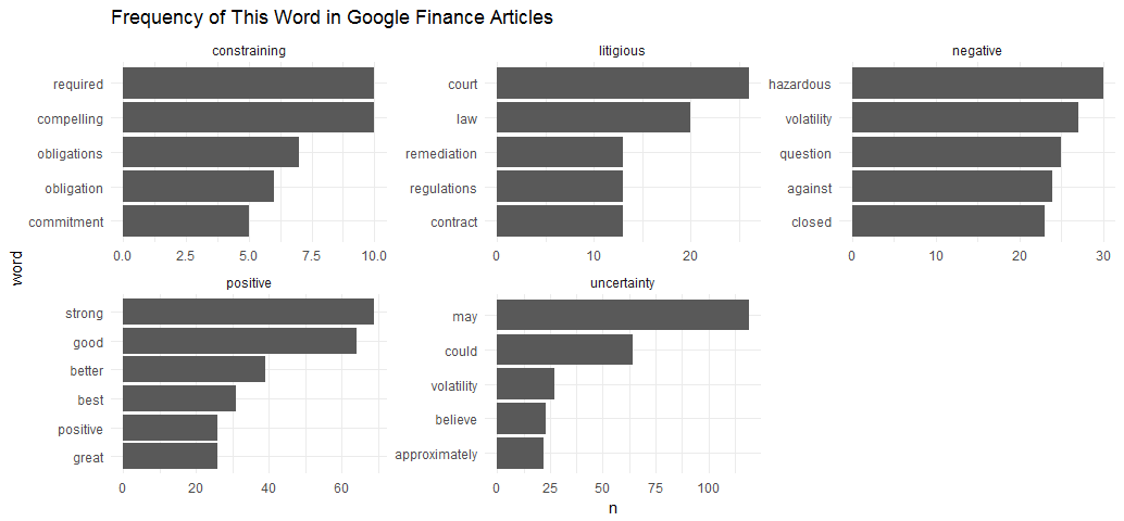
This gives the most common words in the financial news articles associated with each of the six sentiments in the Loughran lexicon. Here I only get five sentiments, this indicates that there is no word can be associated with “superfluous” in recent Google finance news articles related to these four companies.
Now it makes much better sense and I can trust the results to count how frequently each sentiment was associated with each company in these articles.
sentiment_fre <- tokens %>%
  inner_join(get_sentiments("loughran"), by = "word") %>%
  count(sentiment, company) %>%
  spread(sentiment, n, fill = 0)
sentiment_fre
### A tibble: 4 × 6
## company constraining litigious negative positive uncertainty
##* <chr> <dbl> <dbl> <dbl> <dbl> <dbl>
##1 Kraft 10 60 122 97 69
##2 Mondelez 17 3 187 300 155
##3 Starbucks 10 15 246 277 175
##4 Walmart 47 151 230 76 124sentiment_fre %>%
mutate(score = (positive - negative) / (positive + negative)) %>%
mutate(company = reorder(company, score)) %>%
ggplot(aes(company, score, fill = score > 0)) +
geom_col(show.legend = FALSE) +
coord_flip() + theme_minimal() + ggtitle('Positive or Negative Scores Among Recent Google Finance Articles')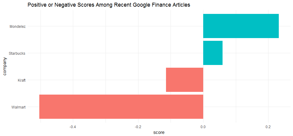
Based the results, I’d say that in May 2017 most of the recent coverage on Walmart was strong negative and most of the recent coverage on Mondelez was positive. A quick search on the recent finance headlines suggests that I am on the right track.
The End
The code to produce all this in R depends heavily on Julia Silge and David Robinson’s Text Mining with R book.