
We are movie-goers, we have heavily relied on how many gold stars a movie gets before we decide whether we watch it or not. I have to admit that we miss good movies sometimes because some critics reviews are controversial, another time we regret after watching a movie because it was not what we expected.
When I was browsing Kaggle dataset, I came across an IMDB movie dataset which contains 5043 movies and 28 variables. Looking at the variables, I think I might be able to find something interesting.
library(ggplot2)
library(dplyr)
library(Hmisc)
library(psych)
movie <- read.csv('movie.csv', stringsAsFactors = F)
str(movie)##'data.frame': 5043 obs. of 28 variables:
## $ color : chr "Color" "Color" "Color" "Color" ...
## $ director_name : chr "James Cameron" "Gore Verbinski" "Sam ##Mendes" "Christopher Nolan" ...
## $ num_critic_for_reviews : int 723 302 602 813 NA 462 392 324 635 375 ...
## $ duration : int 178 169 148 164 NA 132 156 100 141 153 ...
## $ director_facebook_likes : int 0 563 0 22000 131 475 0 15 0 282 ...
## $ actor_3_facebook_likes : int 855 1000 161 23000 NA 530 4000 284 19000 ##10000 ...
## $ actor_2_name : chr "Joel David Moore" "Orlando Bloom" "Rory ##Kinnear" "Christian Bale" ...
## $ actor_1_facebook_likes : int 1000 40000 11000 27000 131 640 24000 799 ##26000 25000 ...
## $ gross : int 760505847 309404152 200074175 448130642 NA ##73058679 336530303 200807262 458991599 301956980 ...
## $ genres : chr "Action|Adventure|Fantasy|Sci-Fi" ##"Action|Adventure|Fantasy" "Action|Adventure|Thriller" "Action|Thriller" ...
## $ actor_1_name : chr "CCH Pounder" "Johnny Depp" "Christoph ##Waltz" "Tom Hardy" ...
## $ movie_title : chr "Avatar " "Pirates of the Caribbean: At ##World's End " "Spectre " "The Dark Knight Rises " ...
## $ num_voted_users : int 886204 471220 275868 1144337 8 212204 ##383056 294810 462669 321795 ...
## $ cast_total_facebook_likes: int 4834 48350 11700 106759 143 1873 46055 2036 ##92000 58753 ...
## $ actor_3_name : chr "Wes Studi" "Jack Davenport" "Stephanie ##Sigman" "Joseph Gordon-Levitt" ...
## $ facenumber_in_poster : int 0 0 1 0 0 1 0 1 4 3 ...
## $ plot_keywords : chr "avatar|future|marine|native|paraplegic" ##"goddess|marriage ceremony|marriage proposal|pirate|singapore" ##"bomb|espionage|sequel|spy|terrorist" ##"deception|imprisonment|lawlessness|police officer|terrorist plot" ...
## $ movie_imdb_link : chr ##"http://www.imdb.com/title/tt0499549/?ref_=fn_tt_tt_1" ##"http://www.imdb.com/title/tt0449088/?ref_=fn_tt_tt_1" ##"http://www.imdb.com/title/tt2379713/?ref_=fn_tt_tt_1" ##"http://www.imdb.com/title/tt1345836/?ref_=fn_tt_tt_1" ...
## $ num_user_for_reviews : int 3054 1238 994 2701 NA 738 1902 387 1117 973 ##...
## $ language : chr "English" "English" "English" "English" ...
## $ country : chr "USA" "USA" "UK" "USA" ...
## $ content_rating : chr "PG-13" "PG-13" "PG-13" "PG-13" ...
## $ budget : num 237000000 300000000 245000000 250000000 NA ##...
## $ title_year : int 2009 2007 2015 2012 NA 2012 2007 2010 2015 ##2009 ...
## $ actor_2_facebook_likes : int 936 5000 393 23000 12 632 11000 553 21000 ##11000 ...
## $ imdb_score : num 7.9 7.1 6.8 8.5 7.1 6.6 6.2 7.8 7.5 7.5 ...
## $ aspect_ratio : num 1.78 2.35 2.35 2.35 NA 2.35 2.35 1.85 2.35 ##2.35 ...
## $ movie_facebook_likes : int 33000 0 85000 164000 0 24000 0 29000 118000 ##10000 ...Always start from the distribution of the data.
ggplot(aes(x = num_critic_for_reviews), data = movie) + geom_histogram(bins = 20, color = 'white') + ggtitle('Histogram of Number of reviews')
summary(movie$num_critic_for_reviews)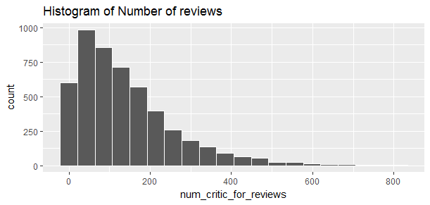
##Min. 1st Qu.  Median    Mean 3rd Qu.    Max.    NA's
##      1      50     110     140     195     813      50
The distribution of the number of reviews is right skewed. Among these 5043 movies, the minimum number of review was 1 and the maximum number of reviews was 813. Majority of the movies received less than 200 reviews.
ggplot(aes(x = imdb_score), data = movie) + geom_histogram(bins = 20, color = 'white') + ggtitle('Histogram of Scores')
summary(movie$imdb_score)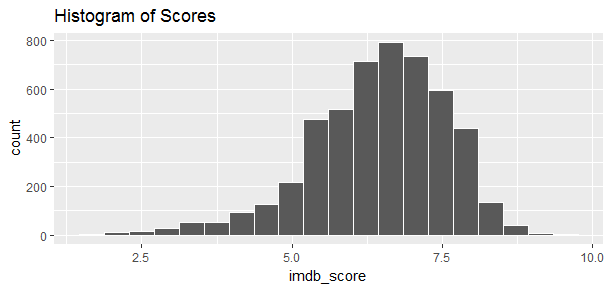
##Min. 1st Qu.  Median    Mean 3rd Qu.    Max.
##   1.60    5.80    6.60    6.44    7.20    9.50
The score distribution is left skewed, with minimum score at 1.60 and maximum score at 9.50.
ggplot(aes(x = title_year), data = movie) + geom_histogram(color='white') +
  ggtitle('Histogram of Title Year')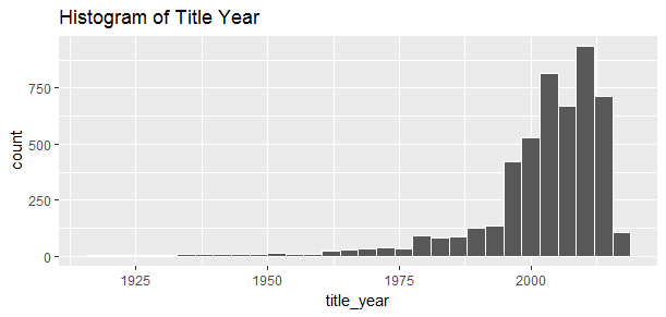
Most of the movies in the dataset were produced after 2000.
boxplot(imdb_score ~ title_year, data=movie, col='indianred')
title("IMDB score vs Title year")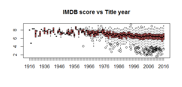
However, the movies with the highest scores were produced in the 1950s, and there have been significant amount of low score movies came out in the recent years.
Which countries produced the most movies and which countries have the highest scores?
country_group <- group_by(movie, country)
movie_by_country <- summarise(country_group,
                               mean_score = mean(imdb_score),
                               n = n())
ggplot(aes(x = country, y = n, fill = country), data = movie_by_country) + geom_bar(stat = 'identity') + theme(legend.position = "none", axis.text=element_text(size=6)) +
  coord_flip() + ggtitle('Countries vs Number of Movies')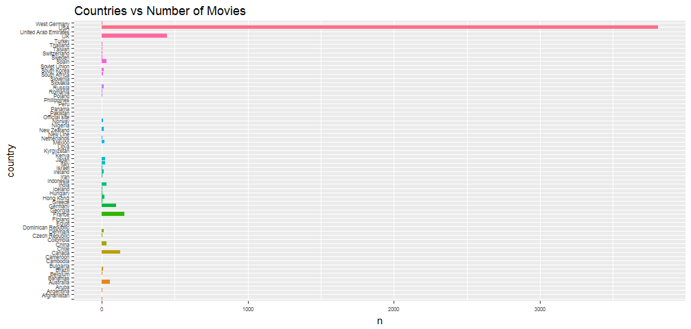
The USA produced the most number of movies.
ggplot(aes(x = country, y = mean_score, fill = country), data = movie_by_country) + geom_bar(stat = 'identity') + theme(legend.position = "none", axis.text=element_text(size=7)) +
  coord_flip() + ggtitle('Countries vs IMDB Scores')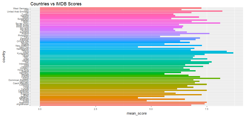
But that does not mean their movie are all good quality. Kyrgyzstan, Libya and United Arab Emirates might have the highest average scores.
Multiple Linear Regression - Variable Selection
Time to do some serious work, I intend to predict IMDB scores from the other variables using multiple linear regression model. Because regression can’t deal with missing values, I will eliminate all missing values by converting to mean or median.
movie$imdb_score <- as.numeric(impute(movie$imdb_score, mean))
movie$num_critic_for_reviews <- as.numeric(impute(movie$num_critic_for_reviews, mean))
movie$duration <- as.numeric(impute(movie$duration, mean))
movie$director_facebook_likes <- as.numeric(impute(movie$director_facebook_likes, mean))
movie$actor_3_facebook_likes <- as.numeric(impute(movie$actor_3_facebook_likes, mean))
movie$actor_1_facebook_likes <- as.numeric(impute(movie$actor_1_facebook_likes, mean))
movie$gross <- as.numeric(impute(movie$gross, mean))
movie$cast_total_facebook_likes <- as.numeric(impute(movie$cast_total_facebook_likes, mean))
movie$facenumber_in_poster <- as.numeric(impute(movie$facenumber_in_poster, mean))
movie$budget <- as.numeric(impute(movie$budget, mean))
movie$title_year <- as.numeric(impute(movie$title_year, median))
movie$actor_2_facebook_likes <- as.numeric(impute(movie$actor_2_facebook_likes, mean))
movie$aspect_ratio <- as.numeric(impute(movie$aspect_ratio, mean))
Now I have got rid of all ‘NA’s. And I picked the following variables as potential candidates for the IMDB score predicators.
- num_critic_for_reviews
- duration
- director_facebook_likes
- actor_1_facebook_likes
- gross
- cast_total_facebook_likes
- facenumber_in_poster
- budget
- movie_facebook_likes
Select a subset of numeric variables for regression modelling.
movie_sub <- subset(movie, select = c(num_critic_for_reviews, duration, director_facebook_likes, actor_1_facebook_likes, gross, cast_total_facebook_likes, facenumber_in_poster, budget, movie_facebook_likes, imdb_score))
pairs.panels(movie_sub, col='red')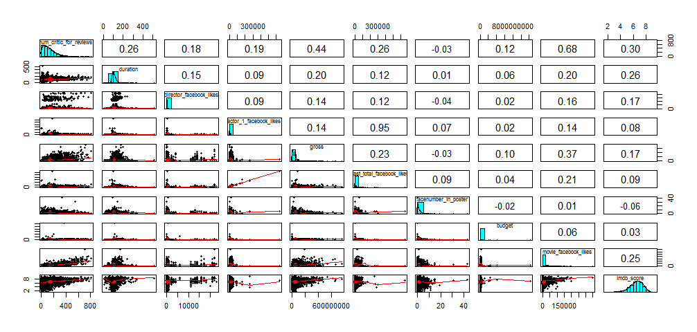
Construct the model
Split data into training and testing.
set.seed(2017)
train_size <- 0.8
train_index <- sample.int(length(movie_sub$imdb_score), length(movie_sub$imdb_score) * train_size)
train_sample <- movie_sub[train_index,]
test_sample <- movie_sub[-train_index,]
Fit the model
I will be using a stepwise selection of variables by backwards elimination. So I start with all candidate varibles and elimiate one at a time.
fit <- lm(imdb_score ~ num_critic_for_reviews + duration +    director_facebook_likes + actor_1_facebook_likes + gross + cast_total_facebook_likes + facenumber_in_poster + budget + movie_facebook_likes, data=train_sample)
summary(fit)
##Call:
##lm(formula = imdb_score ~ num_critic_for_reviews + duration +
## director_facebook_likes + actor_1_facebook_likes + gross +
## cast_total_facebook_likes + facenumber_in_poster + budget +
## movie_facebook_likes, data = train_sample)
##Residuals:
## Min 1Q Median 3Q Max
##-5.088 -0.584 0.085 0.702 3.297
##Coefficients:
## Estimate Std. Error t value
##(Intercept) 5.3211056356832 0.0734493165627 72.45
##num_critic_for_reviews 0.0017938921605 0.0001973870370 9.09
##duration 0.0080649597024 0.0006762454257 11.93
##director_facebook_likes 0.0000392330050 0.0000059815295 6.56
##actor_1_facebook_likes 0.0000138466224 0.0000037417675 3.70
##gross 0.0000000003871 0.0000000002990 1.29
##cast_total_facebook_likes -0.0000123493197 0.0000031674657 -3.90
##facenumber_in_poster -0.0339624416792 0.0083551735721 -4.06
##budget -0.0000000000478 0.0000000000759 -0.63
##movie_facebook_likes 0.0000046436977 0.0000012015153 3.86
## Pr(>|t|)
##(Intercept) < 0.0000000000000002 ***
##num_critic_for_reviews < 0.0000000000000002 ***
##duration < 0.0000000000000002 ***
##director_facebook_likes 0.000000000061 ***
##actor_1_facebook_likes 0.00022 ***
##gross 0.19543
##cast_total_facebook_likes 0.000098245288 ***
##facenumber_in_poster 0.000048983645 ***
##budget 0.52916
##movie_facebook_likes 0.00011 ***
##---
##Signif. codes: 0 ‘***’ 0.001 ‘**’ 0.01 ‘*’ 0.05 ‘.’ 0.1 ‘ ’ 1
##Residual standard error: 1.04 on 4024 degrees of freedom
##Multiple R-squared: 0.143, Adjusted R-squared: 0.141
##F-statistic: 74.8 on 9 and 4024 DF, p-value: <0.0000000000000002I am going to eliminate the variables that has little value, - gross and budget, one at a time, and fit it again.
fit <- lm(imdb_score ~ num_critic_for_reviews + duration + budget +   director_facebook_likes + actor_1_facebook_likes + cast_total_facebook_likes + facenumber_in_poster + movie_facebook_likes, data=train_sample)
summary(fit)
fit <- lm(imdb_score ~ num_critic_for_reviews + duration + director_facebook_likes + actor_1_facebook_likes + cast_total_facebook_likes + facenumber_in_poster + movie_facebook_likes, data=train_sample)
summary(fit) This is the final summary:
##Call:
##lm(formula = imdb_score ~ num_critic_for_reviews + duration +
##    director_facebook_likes + actor_1_facebook_likes + ##cast_total_facebook_likes +
##    facenumber_in_poster + movie_facebook_likes, data = train_sample)

##Residuals:
##   Min     1Q Median     3Q    Max
##-5.080 -0.584  0.079  0.702  3.308

##Coefficients:
##                             Estimate  Std. Error t value             Pr(>|t|)
##(Intercept)                5.32209746  0.07343556   72.47 < 0.0000000000000002 ##***
##num_critic_for_reviews     0.00184176  0.00019151    9.62 < 0.0000000000000002 ##***
##duration                   0.00811866  0.00067383   12.05 < 0.0000000000000002 ##***
##director_facebook_likes    0.00003957  0.00000598    6.62        0.00000000004 ##***
##actor_1_facebook_likes     0.00001304  0.00000369    3.54              0.00041 ##***
##cast_total_facebook_likes -0.00001156  0.00000310   -3.72              0.00020 ##***
##facenumber_in_poster      -0.03422551  0.00834960   -4.10        0.00004230054 ##***
##movie_facebook_likes       0.00000478  0.00000120    3.99        0.00006632357 ##***
##---
##Signif. codes:  0 ‘***’ 0.001 ‘**’ 0.01 ‘*’ 0.05 ‘.’ 0.1 ‘ ’ 1

##Residual standard error: 1.04 on 4026 degrees of freedom
##Multiple R-squared:  0.143,	Adjusted R-squared:  0.141
##F-statistic: 95.9 on 7 and 4026 DF,  p-value: <0.0000000000000002
From the fitted model, I find that the model is significant since the p-value is very small. The “cast_total_facebook_likes” and “facenumber_in_poster” has negative weight. This model has multiple R-squared score of 0.143, meaning that around 14.3% of the variability can be explained by this model.
Let me make a few plots of the model I arrived at.
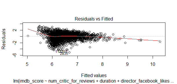
If I consider IMDB scores of all movies in the dataset, it is a non-linear fit, it has a small degree of nonlinearity.
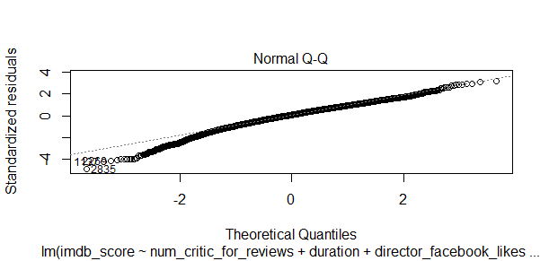
This charts shows how all of the examples of residuals compare against theoretical distances from the model. I can see I have a bit problems here because some of the observations are not neatly fit the line.
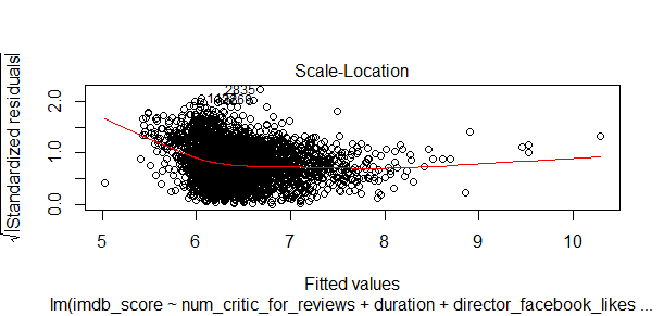
This chart shows the distribution of residuals around the linear model in relation to the IMDB scores of all movies in my data. The higher the score, the less movies, and most movies are in the low or median score range.
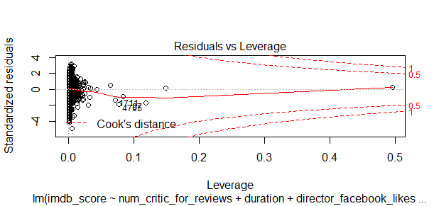
This chart identifies all extrme values, but I don’t see any extrme value has huge impact on my model.
At this point, I think this model is as good as I can get. Let’s evaluate it.
train_sample$pred_score <- predict(fit, newdata = subset(train_sample, select=c(imdb_score, num_critic_for_reviews, duration, director_facebook_likes, actor_1_facebook_likes, cast_total_facebook_likes, facenumber_in_poster, movie_facebook_likes)))
test_sample$pred_score <- predict(fit, newdata = subset(test_sample, select=c(imdb_score, num_critic_for_reviews, duration, director_facebook_likes, actor_1_facebook_likes, cast_total_facebook_likes, facenumber_in_poster, movie_facebook_likes)))
The theoretical model performance is defined here as R-Squared
##Call:
##lm(formula = imdb_score ~ num_critic_for_reviews + duration +
##    director_facebook_likes + actor_1_facebook_likes + ##cast_total_facebook_likes +
##    facenumber_in_poster + movie_facebook_likes, data = train_sample)

##Residuals:
##   Min     1Q Median     3Q    Max
##-5.080 -0.584  0.079  0.702  3.308

##Coefficients:
##                             Estimate  Std. Error t value             Pr(>|t|)
##(Intercept)                5.32209746  0.07343556   72.47 < 0.0000000000000002 ##***
##num_critic_for_reviews     0.00184176  0.00019151    9.62 < 0.0000000000000002 ##***
##duration                   0.00811866  0.00067383   12.05 < 0.0000000000000002 ##***
##director_facebook_likes    0.00003957  0.00000598    6.62        0.00000000004 ##***
##actor_1_facebook_likes     0.00001304  0.00000369    3.54              0.00041 ##***
##cast_total_facebook_likes -0.00001156  0.00000310   -3.72              0.00020 ##***
##facenumber_in_poster      -0.03422551  0.00834960   -4.10        0.00004230054 ##***
##movie_facebook_likes       0.00000478  0.00000120    3.99        0.00006632357 ##***
##---
##Signif. codes:  0 ‘***’ 0.001 ‘**’ 0.01 ‘*’ 0.05 ‘.’ 0.1 ‘ ’ 1

##Residual standard error: 1.04 on 4026 degrees of freedom
##Multiple R-squared:  0.143,	Adjusted R-squared:  0.141
##F-statistic: 95.9 on 7 and 4026 DF,  p-value: <0.0000000000000002
Check how good the model is on the training set.
train_corr <- round(cor(train_sample$pred_score, train_sample$imdb_score), 2)
train_rmse <- round(sqrt(mean((train_sample$pred_score - train_sample$imdb_score)^2)))
train_mae <- round(mean(abs(train_sample$pred_score - train_sample$imdb_score)))
c(train_corr^2, train_rmse, train_mae)
##[1] 0.1444 1.0000 1.0000The correlation between predicted score and actual score for the training set is 14.44%, which is very close to theoretical R-Squared for the model, this is good news. However, on average, on the set of the observations I have previously seen, I am going to make 1 score difference when estimating.
Check how good the model is on the test set.
test_corr <- round(cor(test_sample$pred_score, test_sample$imdb_score), 2)
test_rmse <- round(sqrt(mean((test_sample$pred_score - test_sample$imdb_score)^2)))
test_mae <- round(mean(abs(test_sample$pred_score - test_sample$imdb_score)))
c(test_corr^2, test_rmse, test_mae)
##[1] 0.1521 1.0000 1.0000This result is not bad, the results of the test set are not far from the results of the training set.
Conclusion
- The most important factor that affect movie score is the duration, the longer the movie, the higher the sore will be.
- The number of critic reviews is important, the more reviews a movie receives, the higher the score will be.
- The face number in poster has a negative effect to the movie score. The more faces in a movie poster, the lower the score will be.
The End
I hope movie will be the same after I learn how to analyze movie data. Apprécier le film!
Source code that created this post can be found here. I am happy to hear any feedback and questions.