
The dataset is originally from the National Institute of Diabetes and Digestive and Kidney Diseases. I downloaded from UCI Machine Learning Repository. The objective is to predict based on diagnostic measurements whether a patient has diabetes.
library(ggplot2)
library(dplyr)
library(gridExtra)
library(corrplot)
Look at the structure and the first few rows.
diabetes <- read.csv('diabetes.csv')
dim(diabetes)
str(diabetes)
head(diabetes)
##[1] 768 9
##'data.frame': 768 obs. of 9 variables:
## $ Pregnancies : int 6 1 8 1 0 5 3 10 2 8 ...
## $ Glucose : int 148 85 183 89 137 116 78 115 197 125 ...
## $ BloodPressure : int 72 66 64 66 40 74 50 0 70 96 ...
## $ SkinThickness : int 35 29 0 23 35 0 32 0 45 0 ...
## $ Insulin : int 0 0 0 94 168 0 88 0 543 0 ...
## $ BMI : num 33.6 26.6 23.3 28.1 43.1 25.6 31 35.3 30.5 0 ##...
## $ DiabetesPedigreeFunction: num 0.627 0.351 0.672 0.167 2.288 ...
## $ Age : int 50 31 32 21 33 30 26 29 53 54 ...
## $ Outcome : int 1 0 1 0 1 0 1 0 1 1 ...
## Pregnancies Glucose BloodPressure SkinThickness Insulin BMI
##1 6 148 72 35 0 33.6
##2 1 85 66 29 0 26.6
##3 8 183 64 0 0 23.3
##4 1 89 66 23 94 28.1
##5 0 137 40 35 168 43.1
##6 5 116 74 0 0 25.6
## DiabetesPedigreeFunction Age Outcome
##1 0.627 50 1
##2 0.351 31 0
##3 0.672 32 1
##4 0.167 21 0
##5 2.288 33 1
##6 0.201 30 0Exploratory Data Analysis and Feature Selection
Check missing values
cat("Number of missing value:", sum(is.na(diabetes)), "\n")##Number of missing value: 0Staitstical summary
summary(diabetes)## Pregnancies Glucose BloodPressure SkinThickness Insulin
## Min.: 0.000 Min. : 0.0 Min. : 0.00 Min. : 0.00 Min. : 0.0
## 1st Qu.:1.000 1st Qu.: 99.0 1st Qu.: 62.00 1st Qu.: 0.00 1st Qu.: 0.0 ##Median : 3.000 Median :117.0 Median : 72.00 Median :23.00 Median :30.5 ## Mean : 3.845 Mean :120.9 Mean : 69.11 Mean :20.54 Mean :79.8 ##3rd Qu.: 6.000 3rd Qu.:140.2 3rd Qu.: 80.00 3rd Qu.:32.00 3rd Qu.:127.2 ##Max. :17.000 Max. :199.0 Max. :122.00 Max. :99.00 Max. :846.0
## BMI DiabetesPedigreeFunction Age Outcome
## Min. : 0.00 Min. :0.0780 Min. :21.00 Min. :0.000
## 1st Qu.:27.30 1st Qu.:0.2437 1st Qu.:24.00 1st Qu.:0.000
## Median :32.00 Median :0.3725 Median :29.00 Median :0.000
## Mean :31.99 Mean :0.4719 Mean :33.24 Mean :0.349
## 3rd Qu.:36.60 3rd Qu.:0.6262 3rd Qu.:41.00 3rd Qu.:1.000
## Max. :67.10 Max. :2.4200 Max. :81.00 Max. :1.000 Histogram of numeric variables
p1 <- ggplot(diabetes, aes(x=Pregnancies)) + ggtitle("Number of times pregnant") +
  geom_histogram(aes(y = 100*(..count..)/sum(..count..)), binwidth = 1, colour="black", fill="white") + ylab("Percentage")
p2 <- ggplot(diabetes, aes(x=Glucose)) + ggtitle("Glucose") +
  geom_histogram(aes(y = 100*(..count..)/sum(..count..)), binwidth = 5, colour="black", fill="white") + ylab("Percentage")
p3 <- ggplot(diabetes, aes(x=BloodPressure)) + ggtitle("Blood Pressure") +
  geom_histogram(aes(y = 100*(..count..)/sum(..count..)), binwidth = 2, colour="black", fill="white") + ylab("Percentage")
p4 <- ggplot(diabetes, aes(x=SkinThickness)) + ggtitle("Skin Thickness") +
  geom_histogram(aes(y = 100*(..count..)/sum(..count..)), binwidth = 2, colour="black", fill="white") + ylab("Percentage")
p5 <- ggplot(diabetes, aes(x=Insulin)) + ggtitle("Insulin") +
  geom_histogram(aes(y = 100*(..count..)/sum(..count..)), binwidth = 20, colour="black", fill="white") + ylab("Percentage")
p6 <- ggplot(diabetes, aes(x=BMI)) + ggtitle("Body Mass Index") +
  geom_histogram(aes(y = 100*(..count..)/sum(..count..)), binwidth = 1, colour="black", fill="white") + ylab("Percentage")
p7 <- ggplot(diabetes, aes(x=DiabetesPedigreeFunction)) + ggtitle("Diabetes Pedigree Function") +
  geom_histogram(aes(y = 100*(..count..)/sum(..count..)), colour="black", fill="white") + ylab("Percentage")
p8 <- ggplot(diabetes, aes(x=Age)) + ggtitle("Age") +
  geom_histogram(aes(y = 100*(..count..)/sum(..count..)), binwidth=1, colour="black", fill="white") + ylab("Percentage")
grid.arrange(p1, p2, p3, p4, p5, p6, p7, p8, ncol=2)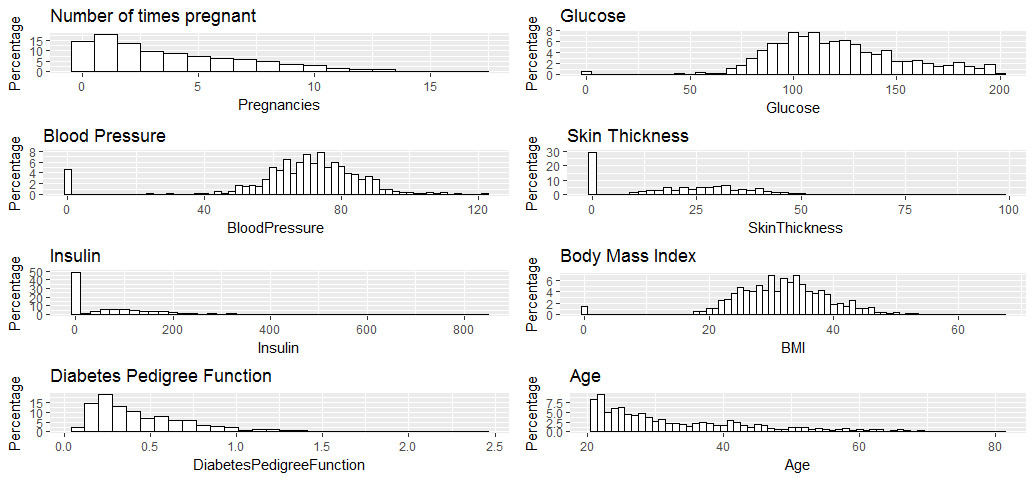
All the variables seem to have reasonable broad distribution, therefore, will be kept for the regression analysis.
Correlation Between Numeric Varibales
numeric.var <- sapply(diabetes, is.numeric)
corr.matrix <- cor(diabetes[,numeric.var])
corrplot(corr.matrix, main="\n\nCorrelation Plot for Numerical Variables", order = "hclust", tl.col = "black", tl.srt=45, tl.cex=0.5, cl.cex=0.5)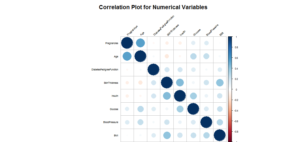
The numeric variabls are almost not correlated.
Correlation bewteen numeric variables and outcome.
attach(diabetes)
par(mfrow=c(2,4))
boxplot(Pregnancies~Outcome, main="No. of Pregnancies vs. Diabetes",
        xlab="Outcome", ylab="Pregnancies")
boxplot(Glucose~Outcome, main="Glucose vs. Diabetes",
        xlab="Outcome", ylab="Glucose")
boxplot(BloodPressure~Outcome, main="Blood Pressure vs. Diabetes",
        xlab="Outcome", ylab="Blood Pressure")
boxplot(SkinThickness~Outcome, main="Skin Thickness vs. Diabetes",
        xlab="Outcome", ylab="Skin Thickness")
boxplot(Insulin~Outcome, main="Insulin vs. Diabetes",
        xlab="Outcome", ylab="Insulin")
boxplot(BMI~Outcome, main="BMI vs. Diabetes",
        xlab="Outcome", ylab="BMI")
boxplot(DiabetesPedigreeFunction~Outcome, main="Diabetes Pedigree Function vs. Diabetes", xlab="Outcome", ylab="DiabetesPedigreeFunction")
boxplot(Age~Outcome, main="Age vs. Diabetes",
        xlab="Outcome", ylab="Age")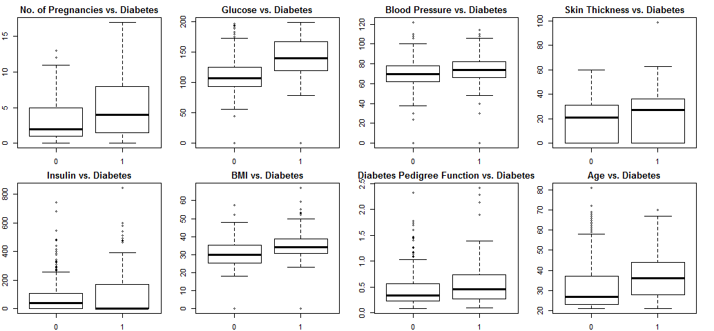
Blood pressure and skin thickness show little variation with diabetes, they will be excluded from the model. Other variables show more or less correlation with diabetes, so will be kept.
Logistic Regression
diabetes$BloodPressure <- NULL
diabetes$SkinThickness <- NULL
train <- diabetes[1:540,]
test <- diabetes[541:768,]
model <-glm(Outcome ~.,family=binomial(link='logit'),data=train)
summary(model)
##Call:
##glm(formula = Outcome ~ ., family = binomial(link = "logit"),
## data = train)
##Deviance Residuals:
## Min 1Q Median 3Q Max
##-2.4366 -0.7741 -0.4312 0.8021 2.7310
##Coefficients:
## Estimate Std. Error z value Pr(>|z|)
##(Intercept) -8.3461752 0.8157916 -10.231 < 2e-16 ***
##Pregnancies 0.1246856 0.0373214 3.341 0.000835 ***
##Glucose 0.0315778 0.0042497 7.431 1.08e-13 ***
##Insulin -0.0013400 0.0009441 -1.419 0.155781
##BMI 0.0881521 0.0164090 5.372 7.78e-08 ***
##DiabetesPedigreeFunction 0.9642132 0.3430094 2.811 0.004938 **
##Age 0.0018904 0.0107225 0.176 0.860053
##---
##Signif. codes: 0 ‘***’ 0.001 ‘**’ 0.01 ‘*’ 0.05 ‘.’ 0.1 ‘ ’ 1
##(Dispersion parameter for binomial family taken to be 1)
## Null deviance: 700.47 on 539 degrees of freedom
##Residual deviance: 526.56 on 533 degrees of freedom
##AIC: 540.56
##Number of Fisher Scoring iterations: 5The top three most relevant features are “Glucose”, “BMI” and “Number of times pregnant” because of the low p-values.
“Insulin” and “Age” appear not statistically significant.
anova(model, test="Chisq")##Analysis of Deviance Table
##Model: binomial, link: logit
##Response: Outcome
##Terms added sequentially (first to last)
## Df Deviance Resid. Df Resid. Dev Pr(>Chi)
##NULL 539 700.47
##Pregnancies 1 26.314 538 674.16 2.901e-07 ***
##Glucose 1 102.960 537 571.20 < 2.2e-16 ***
##Insulin 1 0.062 536 571.14 0.803341
##BMI 1 36.135 535 535.00 1.841e-09 ***
##DiabetesPedigreeFunction 1 8.414 534 526.59 0.003723 **
##Age 1 0.031 533 526.56 0.860201
##---
##Signif. codes: 0 ‘***’ 0.001 ‘**’ 0.01 ‘*’ 0.05 ‘.’ 0.1 ‘ ’ 1From the table of deviance, we can see that adding insulin and age have little effect on the residual deviance.
Cross Validation
fitted.results <- predict(model,newdata=test,type='response')
fitted.results <- ifelse(fitted.results > 0.5,1,0)
misClasificError <- mean(fitted.results != test$Outcome)
print(paste('Accuracy',1-misClasificError))
##[1] "Accuracy 0.789473684210526"Decision Tree
library(rpart)
model2 <- rpart(Outcome ~ Pregnancies + Glucose + BMI + DiabetesPedigreeFunction, data=train,method="class")
plot(model2, uniform=TRUE,
  	main="Classification Tree for Diabetes")
text(model2, use.n=TRUE, all=TRUE, cex=.8)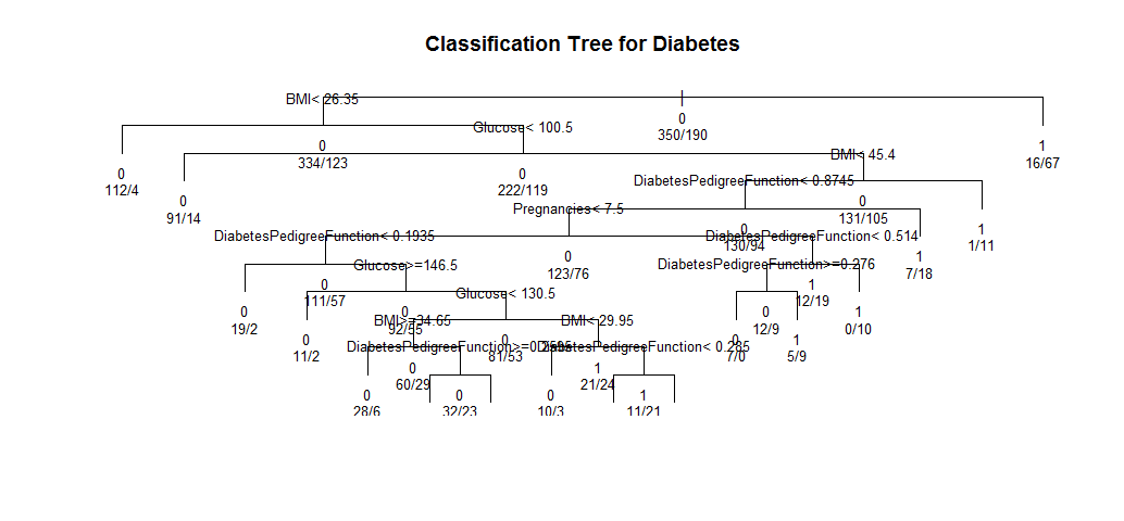
This means if a person’s BMI less than 45.4 and her diabetes digree function less than 0.8745, then she is more likely to have diabetes.
Confusion table and accuracy
treePred <- predict(model2, test, type = 'class')
table(treePred, test$Outcome)
mean(treePred==test$Outcome)
##treePred 0 1
## 0 121 29
## 1 29 49
##[1] 0.745614In this project, I compared the performance of Logistic Regression and Decision Tree algorithms and found that Logistic Regression performed better on this standard, unaltered dataset. However, there are things we can do to improve the generalization performance in decision tree induction such as pruning. I will perform that in the future posts.
Source code that created this post can be found here. I am happy to hear any feedback or questions.