
The Ames Housing dataset was downloaded from kaggle. It is a playground competition’s dataset and my taske is to predict house prices based on house-level features using multiple linear regression model in R.
Prepare the data
library(Hmisc)
library(psych)
library(car)
Split the data into a training set and a testing set.
house <- read.csv('house.csv')
set.seed(2017)
split <- sample(seq_len(nrow(house)), size = floor(0.75 * nrow(house)))
train <- house[split, ]
test <- house[-split, ]
dim(train)
##[1] 1095 81The training set contains 1095 observations and 81 variables. To start, I will hypothesize the following subset of the variables as potential predicators.
-
salePrice - the property’s sale price in dollars. This is the target variable that I am trying to predict.
-
OverallCond - Overall condition rating
-
YearBuilt - Original construction date
-
YearRemodAdd - Remodel data
-
BedroomAbvGr - Number of bedrooms above basement level
-
GrLivArea - Above grade (ground) living area square feet
-
KitchenAbvGr - Number of kitchens above grade
-
TotRmsAbvGrd - Total rooms above grade (does not include bathrooms)
-
GarageCars - Size of garage in car capacity
-
PoolArea - Pool area in square feet
-
LotArea - Lot size in square feet
Construct a new data fram consisting solely of these variables.
train <- subset(train, select=c(SalePrice, LotArea, PoolArea, GarageCars, TotRmsAbvGrd, KitchenAbvGr, GrLivArea, BedroomAbvGr, YearRemodAdd, YearBuilt, OverallCond))
head(train)
## SalePrice LotArea PoolArea GarageCars TotRmsAbvGrd KitchenAbvGr GrLivArea
##1350 122000 5250 0 0 8 1 2358
##784 165500 9101 0 2 4 1 1110
##685 221000 16770 0 2 7 1 1839
##421 206300 7060 0 4 8 2 1344
##1122 212900 10084 0 3 7 1 1552
##1125 163900 9125 0 2 7 1 1482
## BedroomAbvGr YearRemodAdd YearBuilt OverallCond
##1350 4 1987 1872 5
##784 1 1978 1978 6
##685 4 1998 1998 5
##421 2 1998 1997 5
##1122 3 2006 2005 5
##1125 3 1992 1992 5Report variables with missing values.
sapply(train, function(x) sum(is.na(x)))##SalePrice LotArea PoolArea GarageCars TotRmsAbvGrd KitchenAbvGr
## 0 0 0 0 0 0
## GrLivArea BedroomAbvGr YearRemodAdd YearBuilt OverallCond
## 0 0 0 0 0 Summary statistics
summary(train)## SalePrice LotArea PoolArea GarageCars
## Min. : 34900 Min. : 1300 Min. : 0.000 Min. :0.000
## 1st Qu.:129000 1st Qu.: 7500 1st Qu.: 0.000 1st Qu.:1.000
## Median :164000 Median : 9452 Median : 0.000 Median :2.000
## Mean :181598 Mean : 10467 Mean : 3.679 Mean :1.764
## 3rd Qu.:215600 3rd Qu.: 11500 3rd Qu.: 0.000 3rd Qu.:2.000
## Max. :745000 Max. :215245 Max. :738.000 Max. :4.000
## TotRmsAbvGrd KitchenAbvGr GrLivArea BedroomAbvGr YearRemodAdd
## Min. : 2.000 Min. :0.000 Min. : 334 Min. :0.000 Min. :1950
## 1st Qu.:5.000 1st Qu.:1.000 1st Qu.:1124 1st Qu.:2.000 1st Qu.:1967
## Median :6.000 Median :1.000 Median :1458 Median :3.000 Median :1994
## Mean :6.493 Mean :1.045 Mean :1510 Mean :2.848 Mean :1985
## 3rd Qu.:7.000 3rd Qu.:1.000 3rd Qu.:1779 3rd Qu.:3.000 3rd Qu.:2004
## Max. :12.000 Max. :3.000 Max. :5642 Max. :6.000 Max. :2010
## YearBuilt OverallCond
## Min. :1872 Min. :1.000
## 1st Qu.:1954 1st Qu.:5.000
## Median :1974 Median :5.000
## Mean :1972 Mean :5.555
## 3rd Qu.:2001 3rd Qu.:6.000
## Max. :2009 Max. :9.000 Before fitting my regression model I want to investigate how the variables are related to one another.
pairs.panels(train, col='red')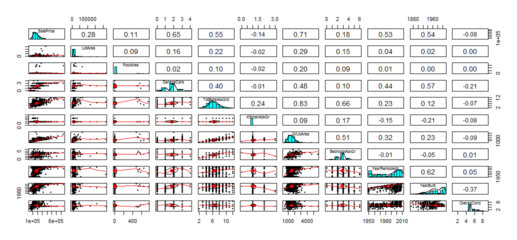
We can see some of the variables are very skewed. If we want to have a good regression model, the varaibles should be normal distributed. The variables should be independent and not correlated. “GrLivArea” and “TotRmsAbvGrd” clearly have a high correlation, I will have to deal with these.
Fit the linear model
fit <-  lm(SalePrice ~ LotArea + PoolArea + GarageCars + TotRmsAbvGrd + KitchenAbvGr + GrLivArea + BedroomAbvGr + YearRemodAdd + YearBuilt + OverallCond, data=train)
summary(fit)
##Call:
##lm(formula = SalePrice ~ LotArea + PoolArea + GarageCars + TotRmsAbvGrd +
## KitchenAbvGr + GrLivArea + BedroomAbvGr + YearRemodAdd +
## YearBuilt + OverallCond, data = train)
##Residuals:
## Min 1Q Median 3Q Max
##-434633 -21648 -3194 16980 294504
##Coefficients:
## Estimate Std. Error t value Pr(>|t|)
##(Intercept) -1.823e+06 1.451e+05 -12.569 < 2e-16 ***
##LotArea 7.174e-01 1.317e-01 5.449 6.28e-08 ***
##PoolArea -1.522e+01 2.777e+01 -0.548 0.5838
##GarageCars 2.107e+04 2.288e+03 9.207 < 2e-16 ***
##TotRmsAbvGrd 6.789e+03 1.672e+03 4.060 5.26e-05 ***
##KitchenAbvGr -4.215e+04 6.195e+03 -6.805 1.67e-11 ***
##GrLivArea 7.598e+01 4.700e+00 16.165 < 2e-16 ***
##BedroomAbvGr -1.605e+04 2.198e+03 -7.303 5.44e-13 ***
##YearRemodAdd 2.115e+02 8.779e+01 2.410 0.0161 *
##YearBuilt 7.235e+02 6.875e+01 10.523 < 2e-16 ***
##OverallCond 7.940e+03 1.356e+03 5.853 6.39e-09 ***
##---
##Signif. codes: 0 ‘***’ 0.001 ‘**’ 0.01 ‘*’ 0.05 ‘.’ 0.1 ‘ ’ 1
##Residual standard error: 41240 on 1084 degrees of freedom
##Multiple R-squared: 0.737, Adjusted R-squared: 0.7346
##F-statistic: 303.7 on 10 and 1084 DF, p-value: < 2.2e-16Interprete the output:
-
R-squred of 0.737 tells us that approximately 74% of variation in sale price can be explained by my model.
-
F-statistics and p-value show the overall significance test of my model.
-
Residual standard error gives an idea on how far observed sale price are from the predicted or fitted sales price.
-
Intercept is the estimated sale price for a house with all the other variables at zero. It does not provide any meaningful interpretation.
-
The slope for “GrlivArea”(7.598e+01) is the effect of Above grade living area square feet on sale price adjusting or controling for the other variables, i.e we associate an increase of 1 square foot in “GrlivArea” with an increase of $75.98 in sale price adjusting or controlling for the other variables.
Stepwise Procedure
Using backward elimination to remove the predictor with the largest p-value over 0.05. In this case, I will remove “PoolArea” first, then fit the model again.
fit <-  lm(SalePrice ~ LotArea + GarageCars + TotRmsAbvGrd + KitchenAbvGr + GrLivArea + BedroomAbvGr + YearRemodAdd + YearBuilt + OverallCond, data=train)
summary(fit)
##Call:
##lm(formula = SalePrice ~ LotArea + GarageCars + TotRmsAbvGrd +
## KitchenAbvGr + GrLivArea + BedroomAbvGr + YearRemodAdd +
## YearBuilt + OverallCond, data = train)
##Residuals:
## Min 1Q Median 3Q Max
##-440086 -21728 -3086 16994 287342
##Coefficients:
## Estimate Std. Error t value Pr(>|t|)
##(Intercept) -1.826e+06 1.449e+05 -12.601 < 2e-16 ***
##LotArea 7.153e-01 1.316e-01 5.437 6.69e-08 ***
##GarageCars 2.114e+04 2.284e+03 9.255 < 2e-16 ***
##TotRmsAbvGrd 6.888e+03 1.662e+03 4.144 3.67e-05 ***
##KitchenAbvGr -4.212e+04 6.192e+03 -6.802 1.70e-11 ***
##GrLivArea 7.543e+01 4.590e+00 16.433 < 2e-16 ***
##BedroomAbvGr -1.608e+04 2.196e+03 -7.321 4.80e-13 ***
##YearRemodAdd 2.135e+02 8.769e+01 2.434 0.0151 *
##YearBuilt 7.231e+02 6.873e+01 10.521 < 2e-16 ***
##OverallCond 7.930e+03 1.356e+03 5.849 6.56e-09 ***
##---
##Signif. codes: 0 ‘***’ 0.001 ‘**’ 0.01 ‘*’ 0.05 ‘.’ 0.1 ‘ ’ 1
##Residual standard error: 41230 on 1085 degrees of freedom
##Multiple R-squared: 0.7369, Adjusted R-squared: 0.7347
##F-statistic: 337.7 on 9 and 1085 DF, p-value: < 2.2e-16After eliminating “PoolArea”, R-Squared almost identical, Adjusted R-squared slightly improved. At this point, I think I can start building the model.
However, as we have seen earlier, two variables - “GrLivArea” and “TotRmsAbvGrd” are highly correlated, the multicollinearity between “GrLivArea” and “TotRmsAbvGrd” means that we should not directly interpret “GrLivArea” as the effect of “GrLivArea” on sale price adjusting for “TotRmsAbvGrd”. These two effects are somewhat bounded together.
attach(train)
cor(GrLivArea, TotRmsAbvGrd, method='pearson')
##[1] 0.826969Create a confidence interval for the model coefficients
confint(fit, conf.level=0.95)## 2.5 % 97.5 %
##(Intercept) -2.110407e+06 -1.541712e+06
##LotArea 4.571854e-01 9.734940e-01
##GarageCars 1.665678e+04 2.561958e+04
##TotRmsAbvGrd 3.626750e+03 1.014894e+04
##KitchenAbvGr -5.426898e+04 -2.996842e+04
##GrLivArea 6.642123e+01 8.443367e+01
##BedroomAbvGr -2.038677e+04 -1.176829e+04
##YearRemodAdd 4.141973e+01 3.855420e+02
##YearBuilt 5.882452e+02 8.579526e+02
##OverallCond 5.269715e+03 1.059089e+04For example, from the 2nd model, I have estimated the slope for “GrLivArea” is 75.43. I am 95% confident that the true slope for “GrLivArea” is between 66.42 and 84.43.
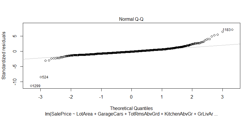
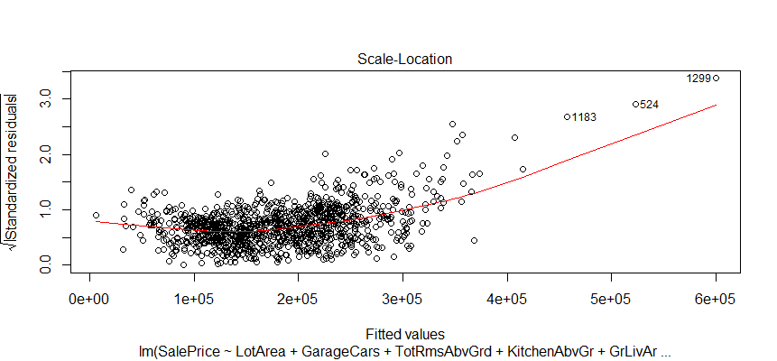
Check the diagnostic plots for the model
plot(fit)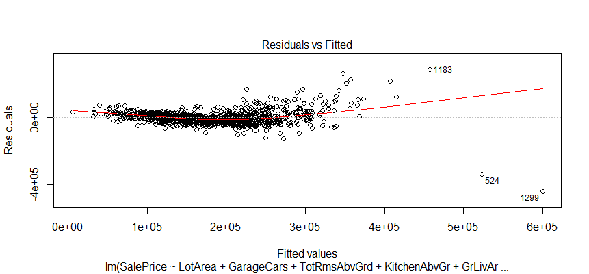
The relationship between predictor variables and an outcome variable is approximate linear. There are three extreme cases (outliers).
It looks like I don’t have to be concerned too much, although two observations numbered as 524 and 1299 look a little off.
The distribution of residuals around the linear model in relation to the sale price. Most of the houses in the data in the lower and median price range, the higher price, the less observations.
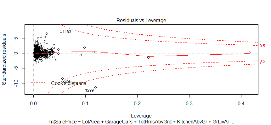
This plot helps us to find influential cases if any. Not all outliers are influential in linear regression analysis. It looks like none of the outliers in my model are influential.
Testing the prediction model
test <- subset(test, select=c(SalePrice, LotArea, GarageCars, TotRmsAbvGrd, KitchenAbvGr, GrLivArea, BedroomAbvGr, YearRemodAdd, YearBuilt, OverallCond))
prediction <- predict(fit, newdata = test)
Look at the first few values of prediction, and compare it to the values of salePrice in the test data set.
head(prediction)## 4 10 16 20 22 34
##176501.95 65626.55 130650.30 135358.79 102336.97 161300.96 head(test$SalePrice)##[1] 140000 118000 132000 139000 139400 165500At last, calculate the value of R-squared for the prediction model on the test data set. In general, R-squared is the metric for evaluating the goodness of fit of my model. Higher is better with 1 being the best.
SSE <- sum((test$SalePrice - prediction) ^ 2)
SST <- sum((test$SalePrice - mean(test$SalePrice)) ^ 2)
1 - SSE/SST
##[1] 0.7421962Source code that created this post can be found here. I am happy to hear any feedback or questions.