
The Gloabl Terrorism database (GDS) is an open-source database including information on terrorist attacks around the world from 1970 through 2015. The dataset I am using contains more than 150,000 terrorism attacks worldwide from 1970 to 2015 except 1993.
terrorism <- read.csv('terrorism.csv', stringsAsFactors = F)There are 137 columns in the dataset, to make it neat, I will have to do some subsetting, only keep the columns I need.
terrorism <- terrorism[,c("iyear","imonth", "iday", "country_txt", "region_txt", "provstate", "city", "latitude", "longitude", "attacktype1_txt", "targtype1_txt", "corp1", "target1", "natlty1_txt", "gname", "weaptype1_txt", "weapsubtype1_txt")]Terrorist Attack Trends
library(ggplot2)
library(dplyr)
library(ggthemes)
by_year <- terrorism %>% group_by(iyear) %>%
  summarise(n=n())
ggplot(aes(x = iyear, y = n), data = by_year) +
        geom_line(size = 2.5, alpha = 0.7, color = "mediumseagreen") +
        geom_point(size = 0.5) + xlab("Year") + ylab("Number of terrorist Attacks") +
        ggtitle("Terrorist Attacks Worldwide by Year 1970-2015") + theme_fivethirtyeight()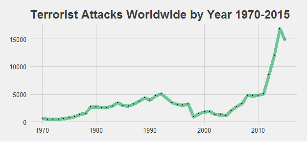
Globally, terrorist attacks have increased dramatically since 2010,
by_region <- terrorism %>% group_by(region_txt, iyear) %>%
  summarise(n=n())
ggplot(by_region, aes(x = iyear, y = n, colour = region_txt)) +
  geom_line() +
  geom_point() +
  facet_wrap(~region_txt) + xlab('Year') +
  ggtitle('Terrorist Attacks by Region and Year 1970-2015') +
  theme(legend.position="none")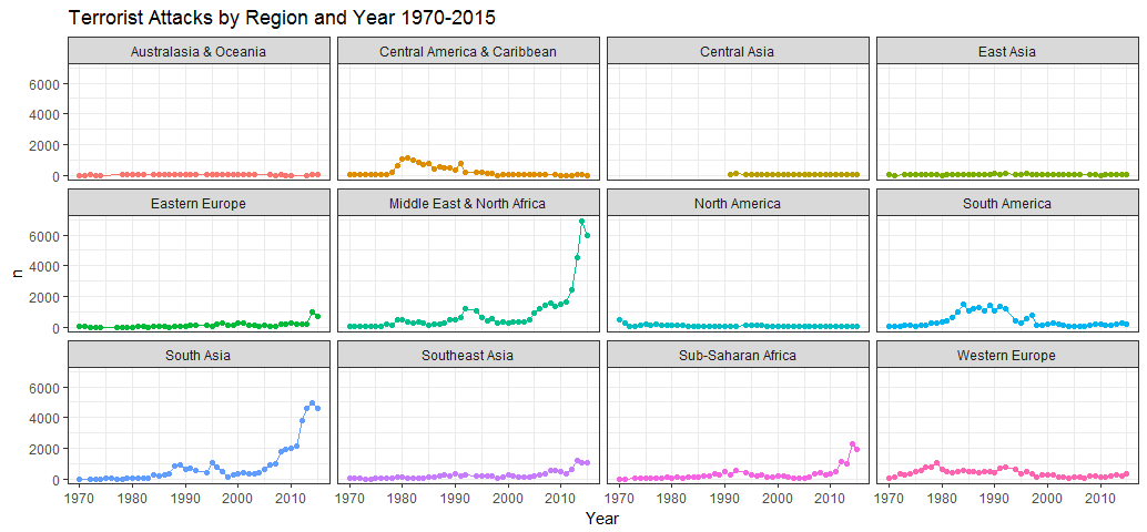
Central America was very unstable starting from the late 1970’s, it got better with time, and it has been stablized since around 1995.
Western Europe had a rough past, experienced many attacks until early 2000s.
South America had the similar pattern, was very dangerous since early 1980 until just before 2000.
Middle East, North Africa and South Asia had a relative quiet past unitl around 1980, the terrorist attacks in those regions had a steady increase from 1980s to around 2005, and had surged dramatically since then.
by_region_no_year <- terrorism %>% group_by(region_txt) %>%
  summarise(n=n())
ggplot(aes(x=reorder(region_txt, n), y=n), data=by_region_no_year) +
  geom_bar(stat = 'identity') +
  ggtitle('Terrorist Attacks by Region 1970-2015') + coord_flip() + theme_fivethirtyeight()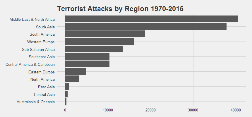
A small fraction of the terrorist attacks happened in the Western countries. Most attacks were heavily concentrated geographically in Middle East, North Africa and South Asia.
Let’s look at the countries.
by_country <- terrorism %>% group_by(country_txt) %>%
  summarise(n=n())
by_country <- arrange(by_country, desc(n))
top10 <- head(by_country, 10)
top10
ggplot(aes(x=reorder(country_txt, n), y=n), data=top10) +
  geom_bar(stat = 'identity') + xlab('Country') + ylab('Number of Terrorist Attacks') + ggtitle('Countries with the most terrorist attacks, 1970-2015') +
  coord_flip() + theme_fivethirtyeight()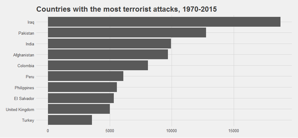
Iraq, Afghanistan and pakistan, India have suffered the most from terrorism. Surprisingly, United Kingdom tops the list in Europe, with almost 5000 attackes from 1970 to 2015.
Tactics and Weapons
by_attacktype <- terrorism %>% group_by(attacktype1_txt) %>%
  summarise(n=n())
ggplot(aes(x=reorder(attacktype1_txt, n), y=n), data=by_attacktype) +
  geom_bar(stat = 'identity') + xlab('Attack Type') + ylab('Number of Attacks') + ggtitle('Terrorist Attack Tactics Wordwide, 1970-2015') + coord_flip() +
  theme_fivethirtyeight()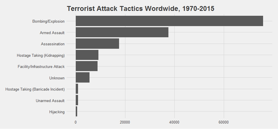
by_weapon <- terrorism %>% group_by(weaptype1_txt) %>%
  summarise(n=n())
ggplot(aes(x=reorder(weaptype1_txt, n), y=n), data=by_weapon) +
  geom_bar(stat = 'identity') + xlab('Weapon') + ylab('Number of Attacks') + ggtitle('Terrorist Attack By Weapon Wordwide, 1970-2015') + coord_flip() +
  theme_fivethirtyeight()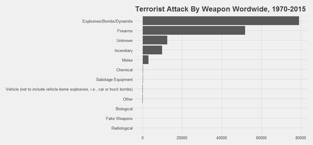
The most commonly used attack tactic from 1970 to 2015 involved bomb and explosives, followed by armed assault.
Let’s look at the most recent year - 2015.
Casualties
To obtain more detailed death information, I went to US Department of State Website download a small dateset with casualty information.
library(xlsx)
library(reshape2)
casualties <- read.xlsx('casualties.xlsx', sheetIndex = 1, header = TRUE, stringsAsFactors = F)
casualties <- melt(casualties, id="month")
casualties<-casualties[!casualties$month=="Total",]
casualties$month <- ordered(casualties$month, levels=c('January', 'February', 'March', 'April', 'May', 'June', 'July', 'August', 'September', 'October', 'November', 'December'))
ggplot(aes(x=month, y=value, fill=variable), data=casualties) +
  geom_bar(stat = 'identity', position = position_dodge()) +
  ggtitle('Terrorist attacks and casualties worldwide by month, 2015') +
  theme_fivethirtyeight()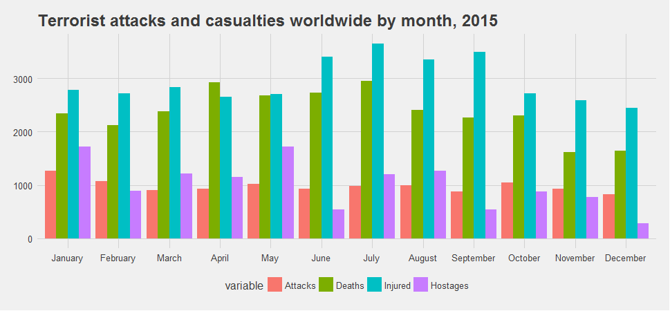
The total number of people killed in terrorist attacks peaked in April and July 2015, and the months with the most combined deaths and injuries were June, July, August, and September, January and May had the most kidnaps.
Perpetrators
Because there were so many unknown values in the original dataset, I have to fetch data again from US Department of State Website about terrorist group information.
group <- read.xlsx('group.xlsx', sheetIndex = 1, header=T, stringsAsFactors=F)
group <- melt(group, id = 'group_name')
group[5, 1] = "Kurdistan Workers' Party"
group[10, 1] = "Kurdistan Workers' Party"
group[15, 1] = "Kurdistan Workers' Party"
group[20, 1] = "Kurdistan Workers' Party"
ggplot(aes(x=group_name, y=value, fill=variable), data=group) +
  geom_bar(stat = 'identity', position = position_dodge()) + ggtitle('Terrorist Groups with the most Attacks Wordwide, 2015') +
  theme(axis.text.x = element_text(angle = 45, hjust = 1))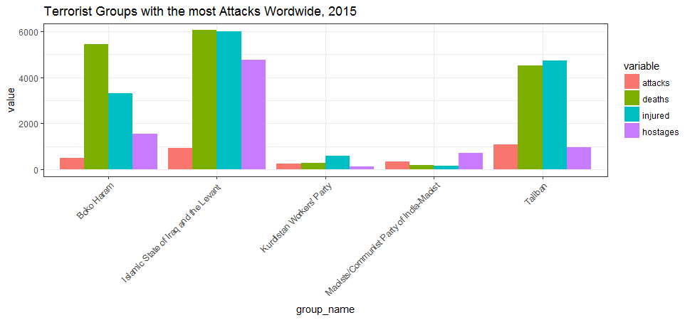
Along with the number of terrorist attacks they carried out, these five terrorist groups were responsible for the most terrorist attacks in 2015. Among those five groups, Islamic State of Iraq and the Levant (ISIL) is world’s deadliest terrorist organization and responsible for more than 6000 deaths in 2015.
Who are they targeting?
attack2015 <- terrorism[terrorism$iyear==2015, ]
by_target <- attack2015 %>% group_by(targtype1_txt) %>%
  summarise(n=n())
by_target <- arrange(by_target, desc(n))
by_target
ggplot(aes(x=reorder(targtype1_txt, n), y=n), data=by_target) +
  geom_bar(stat = 'identity') + ggtitle('Terrorist Attack Targets/Victims, 2015') +
  coord_flip() + theme_fivethirtyeight()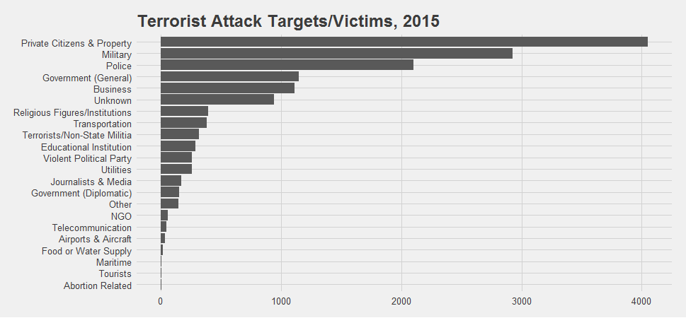
Which countries/cities were the most dangerous in 2015?
attack2015_by_city <- attack2015 %>% group_by(country_txt, city) %>%
  summarise(n=n())
attack2015_by_city <- arrange(attack2015_by_city, desc(n))
top10_city_2015 <- head(attack2015_by_city, 20)
top10_city_2015
## country_txt city n
## <chr> <chr> <int>
##1 Iraq Baghdad 999
##2 Bangladesh Dhaka 210
##3 Afghanistan Unknown 160
##4 Libya Benghazi 150
##5 Pakistan Karachi 143
##6 Yemen Aden 101
##7 Egypt Arish 97
##8 Yemen Sanaa 93
##9 Somalia Mogadishu 92
##10 Yemen Taizz 91
##11 Yemen Unknown 91
##12 Iraq Ramadi 87
##13 Syria Damascus 86
##14 Pakistan Quetta 84
##15 Syria Aleppo 83
##16 Afghanistan Kabul 80
##17 Egypt Sheikh Zuweid 74
##18 Burundi Bujumbura 73
##19 Libya Sirte 69
##20 Iraq Madain 65Baghdad was the most dangerous city in 2015, with approximately 1000 terrorist attacks in one year, but since when it became dangerous?
baghdad <- terrorism[terrorism$city=='Baghdad', ]
baghdad_year <- baghdad %>% group_by(iyear) %>%
  summarise(n=n())
ggplot(aes(x = iyear, y = n), data = baghdad_year) +
        geom_line(size = 2.5, alpha = 0.7, color = "mediumseagreen") +
        geom_point(size = 0.5) + xlab("Year") + ylab("Number of terrorist Attacks") +
        ggtitle("Terrorist Attacks in Baghdad by Year 1970-2015") + theme_fivethirtyeight()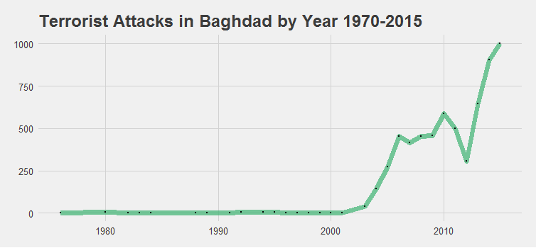
baghdad_type <- baghdad %>% group_by(attacktype1_txt, iyear) %>%
  summarise(n=n())
ggplot(aes(x=iyear, y=n, fill=attacktype1_txt), data=baghdad_type) +
  geom_bar(stat = 'identity') +
  ggtitle('Attack Type in Baghdad') + theme_fivethirtyeight()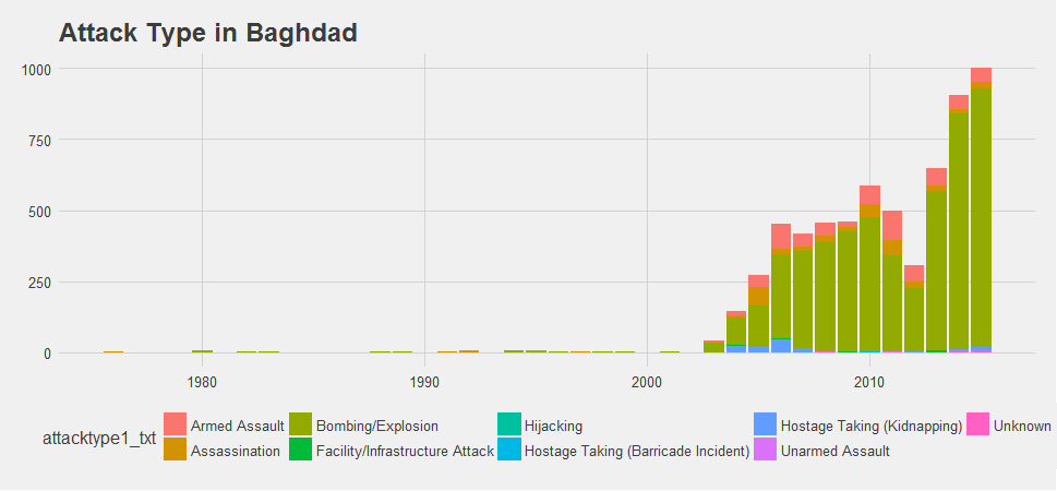
Baghdad once was a prestigious learning and cultural center. Since the coalition invasion in 2003, it has become one of the most dangerous cities on Earth.
A heatmap of terrorist attack deaths worldwide 2015
gtd <- read.csv("terrorism.csv")
gtd2015 <- gtd[gtd$iyear==2015, ]
gtd2015 <- aggregate(nkill~country_txt,gtd2015,sum)
library(rworldmap)
gtdMap <- joinCountryData2Map( gtd2015,
                               nameJoinColumn="country_txt",
                               joinCode="NAME" )

mapDevice('x11')
mapCountryData( gtdMap,
                nameColumnToPlot='nkill',
                catMethod='fixedWidth',
                numCats=100 )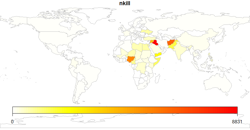
Source code that created this post can be found here. I am happy to hear any feedback or questions.