
Just finished a few hours text mining lesson, can’t wait to put my new skill into practice, starting from Trump’s tweets.
First, apply API keys from twitter.
library(twitteR)
consumer_key <- "Your_Consumer_Key"
consumer_secret <- "Your_Consumer_Secret"
access_token <- NULL
access_secret <- NULL
setup_twitter_oauth(consumer_key, consumer_secret, access_token, access_secret)
The maximize request is 3200 tweets, I got 815, which is not bad.
tweets <- userTimeline("realDonaldTrump", n = 3200)
(n.tweet <- length(tweets))
##[1] 815Have a look the first three, then convert all these 815 tweets to a data frame.
tweets[1:3]
tweets.df <- twListToDF(tweets)
##[[1]]
##[1] "realDonaldTrump: Looking forward to hosting our heroes from the Wounded ##Warrior Project (@WWP) Soldier Ride to the @WhiteHouse on Th… ##https://t.co/QLC0qFD94x"
##[[2]]
##[1] "realDonaldTrump: Getting ready to meet President al-Sisi of Egypt. On ##behalf of the United States, I look forward to a long and wonderful ##relationship."
##[[3]]
##[1] "realDonaldTrump: .@FoxNews from multiple sources: \"There was electronic ##surveillance of Trump, and people close to Trump. This is unprecedented.\" ##@FBI"Text cleaning process, which includes convert all letters to lower case, remove URL, remove anything other than English letter and space, remove stopwords and extra white space.
library(tm)
library(stringr)
myCorpus <- Corpus(VectorSource(tweets.df$text))
myCorpus <- tm_map(myCorpus, content_transformer(str_to_lower))
removeURL <- function(x) gsub("http[^[:space:]]*", "", x)
myCorpus <- tm_map(myCorpus, content_transformer(removeURL))
removeNumPunct <- function(x) gsub("[^[:alpha:][:space:]]*", "", x)
myCorpus <- tm_map(myCorpus, content_transformer(removeNumPunct))
myStopwords <- myStopwords <- c(stopwords('english'), "amp", "trump")
myCorpus <- tm_map(myCorpus, removeWords, myStopwords)
myCorpus <- tm_map(myCorpus, stripWhitespace)
Look at these three tweets again.
myCorpus <- tm_map(myCorpus, stemDocument)
inspect(myCorpus[1:3])
##<<SimpleCorpus>>
##Metadata: corpus specific: 1, document level (indexed): 0
##Content: documents: 3
##[1] look forward host hero wound warrior project wwp soldier ride whitehous th
##[2] get readi meet presid alsisi egypt behalf unit state look forward long ##wonder relationship
##[3] foxnew multipl sourc electron surveil peopl close unpreced fbiNeed to replace a few words, such as “peopl” to “people”, “whitehous” to “whitehouse”, “countri” to “country”.
replaceWord <- function(corpus, oldword, newword) {
  tm_map(corpus, content_transformer(gsub),
         pattern=oldword, replacement=newword)
}
myCorpus <- replaceWord(myCorpus, "peopl", "people")
myCorpus <- replaceWord(myCorpus, "whitehous", "whitehouse")
myCorpus <- replaceWord(myCorpus, "countri", "country")
Building term document matrix
This is a matrix of numbers (0 and 1) that keeps track of which documents in a corpus use which terms.
tdm <- TermDocumentMatrix(myCorpus, control = list(wordLengths = c(1, Inf)))
tdm
##<<TermDocumentMatrix (terms: 2243, documents: 815)>>
##Non-/sparse entries: 8419/1819626
##Sparsity : 100%
##Maximal term length: 29
##Weighting : term frequency (tf)As you can see, the term-document matrix is composed of 2243 terms and 815 documents(tweets). It is very sparse, with 100% of the entries being zero. Let’s have a look at the terms of ‘clinton’, ‘bad’ and ‘great’, and tweets numbered 21 to 30.
idx <- which(dimnames(tdm)$Terms %in% c("clinton", "bad", "great"))
as.matrix(tdm[idx, 21:30])
## Docs
##Terms 21 22 23 24 25 26 27 28 29 30
## clinton 0 0 0 0 0 0 0 0 0 0
## great 0 1 0 0 0 0 0 0 1 1
## bad 0 0 0 0 0 0 0 0 0 0What are the top frequent terms?
(freq.terms <- findFreqTerms(tdm, lowfreq = 40))##[1] "get" "presid" "state" "people" "clinton" "hillari" "just" "big"
##[9] "us" "join" "go" "time" "will" "news" "thank" "now"
##[17] "country" "great" "today" "elect" "job" "watch" "make" "america"
##[25] "pm" "vote"A picture worth a thousand words.
term.freq <- rowSums(as.matrix(tdm))
term.freq <- subset(term.freq, term.freq >= 40)
df <- data.frame(term = names(term.freq), freq = term.freq)
library(ggplot2)
ggplot(df, aes(x=term, y=freq)) + geom_bar(stat="identity") + xlab("Terms") + ylab("Count") + coord_flip() + theme(axis.text=element_text(size=7))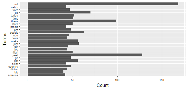
Word Cloud
m <- as.matrix(tdm)
word.freq <- sort(rowSums(m), decreasing = T)
library(RColorBrewer)
pal <- brewer.pal(9, "BuGn")[-(1:4)]
library(wordcloud)
wordcloud(words = names(word.freq), freq = word.freq, min.freq = 3, random.order = F, colors = pal)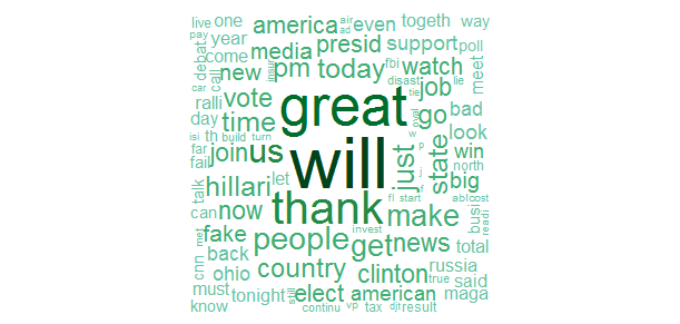
Which word/words are associated with ‘will’?
findAssocs(tdm, "will", 0.2)##$will
## bring dream wealth back togeth god pig
## 0.28 0.27 0.27 0.22 0.22 0.20 0.20 Which word/words are associated with ‘great’? - This is obvious.
findAssocs(tdm, "great", 0.2)##$great
##america make togeth
## 0.35 0.32 0.25Which word/ words are associated with ‘bad’?
findAssocs(tdm, "bad", 0.2)##$bad
## dude stupid judg relationship fool ban
## 0.34 0.34 0.25 0.24 0.24 0.23Clustering Words
tdm2 <- removeSparseTerms(tdm, sparse=0.95)
m2 <- as.matrix(tdm2)
distMatrix <- dist(scale(m2))
fit <- hclust(distMatrix, method="ward.D")
plot(fit)
rect.hclust(fit, k=10)
(groups <- cutree(fit, k=10))
##get presid state people clinton hillari just us join go
##1 1 1 2 3 3 4 5 6 1
##time will news thank now country great today elect watch
## 1 7 4 8 1 2 9 10 1 1
##make america vote
## 1 1 1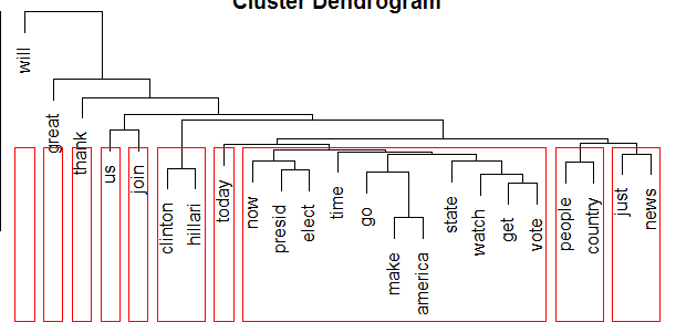
We can see the words in the tweets, words “will, great, thank, us, join, today” are not clustered into any group, “hillari, clinton” are clustered into one group, “now, president, elect, time, go, make, america, state, watch, get, vote” are clustered in one group, “people, country” are clustered into one group, and “just, nows” are clustered into one group.
Clustering Tweets with the k-means Algorithm
m3 <- t(m2)
set.seed(100)
k <- 8
kmeansResult <- kmeans(m3, k)
round(kmeansResult$centers, digits=3)
## get presid state people clinton hillari just us join go time will
##1 0.000 0.042 0.021 0.729 0.000 0.021 0.167 0.021 0.000 0.083 0.042 0.021
##2 0.027 0.068 0.000 0.000 0.057 0.000 0.070 0.000 0.000 0.043 0.062 0.000
##3 0.100 0.036 0.027 0.091 0.009 0.009 0.045 0.000 0.009 0.073 0.082 1.209
##4 0.047 0.093 0.023 0.070 0.395 1.047 0.093 0.000 0.000 0.070 0.023 0.116
##5 0.146 0.042 0.115 0.125 0.010 0.000 0.052 0.021 0.000 0.115 0.073 0.146
##6 0.130 0.037 0.000 0.000 0.000 0.037 0.056 1.093 0.019 0.056 0.037 0.185
##7 0.023 0.000 0.000 0.000 0.000 0.000 0.047 0.163 1.000 0.000 0.047 0.070
##8 0.212 0.038 0.654 0.058 0.077 0.019 0.077 0.019 0.000 0.058 0.096 0.038
## news thank now country great today elect watch make america vote
##1 0.042 0.021 0.021 0.542 0.021 0.042 0.083 0.062 0.042 0.000 0.062
##2 0.073 0.119 0.068 0.000 0.000 0.060 0.068 0.054 0.027 0.019 0.000
##3 0.027 0.118 0.027 0.055 0.136 0.055 0.027 0.055 0.073 0.027 0.027
##4 0.000 0.000 0.047 0.000 0.000 0.023 0.047 0.000 0.000 0.000 0.023
##5 0.104 0.240 0.073 0.042 1.125 0.135 0.031 0.083 0.323 0.281 0.052
##6 0.019 0.185 0.074 0.185 0.074 0.019 0.000 0.000 0.074 0.037 0.019
##7 0.000 0.023 0.047 0.000 0.000 0.023 0.000 0.070 0.000 0.047 0.023
##8 0.019 0.135 0.038 0.038 0.000 0.115 0.115 0.058 0.019 0.019 0.635Check the top three words in every cluster
for (i in 1:k) {
cat(paste("cluster ", i, ": ", sep=""))
s <- sort(kmeansResult$centers[i,], decreasing=T)
cat(names(s)[1:3], "\n")
}
##cluster 1: people country just
##cluster 2: thank news just
##cluster 3: will great thank
##cluster 4: hillari clinton will
##cluster 5: great make america
##cluster 6: us will thank
##cluster 7: join us will
##cluster 8: state vote get I have admit that I can’t easily distinguish cluster 2, cluster 3 and cluster 6 of Trump’s tweets are of different topics.
Sentiment Analysis
The sentiment analysis algorithm used here is based on NRC Word Emotion Association Lexion, available from the tidytext package which developed by Julia Silge and David Robinson. The algorithm associates with eight basic emotions (anger, fear, anticipation, trust, surprise, sadness, joy, and disgust) and two sentiments (negative and positive).
Sometimes there are tweaks I need to do to get rid of the problem characters.
library(tidytext)
library(syuzhet)
tweets.df$text <- sapply(tweets.df$text,function(row) iconv(row, "latin1", "ASCII", sub=""))
Trump_sentiment <- get_nrc_sentiment(tweets.df$text)
Have a look the head of Trump’s tweets sentiment scores:
head(Trump_sentiment)##anger anticipation disgust fear joy sadness surprise trust negative positive
##1 2 0 0 1 0 1 0 0 0 3
##2 0 2 0 0 1 0 1 3 0 4
##3 0 0 0 1 0 0 2 0 0 0
##4 0 1 0 0 1 1 1 1 0 3
##5 1 1 1 0 1 0 1 2 1 2
##6 0 0 0 0 0 0 0 1 1 2Then combine Trump tweets dataframe and Trump sentiment dataframe together.
tweets.df <- cbind(tweets.df, Trump_sentiment)
sentiment_total <- data.frame(colSums(tweets.df[,c(17:26)]))
names(sentiment_total) <- "count"
sentiment_total <- cbind("sentiment" = rownames(sentiment_total), sentiment_total)
Let’s visualize it!
ggplot(aes(x = sentiment, y = count, fill = sentiment), data = sentiment_total) +
  geom_bar(stat = 'identity') + ggtitle('Sentiment Score for Trump Latest Tweets') + theme(legend.position = "none")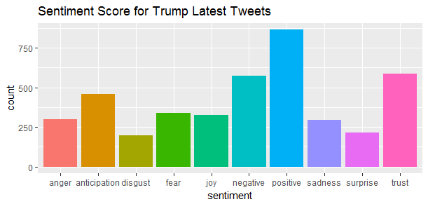
Trump’s tweets appear more positive than negative, more trust than anger. Has Trump’s tweets always been positive or only after he won the election?
library(dplyr)
library(lubridate)
library(reshape2)
tweets.df$timestamp <- with_tz(ymd_hms(tweets.df$created), "America/New_York")
Tweets_trend <- tweets.df %>%
        group_by(timestamp = cut(timestamp, breaks="1 months")) %>%
        summarise(negative = mean(negative),
                  positive = mean(positive)) %>% melt
library(scales)
ggplot(aes(x = as.Date(timestamp), y = value, group = variable), data = Tweets_trend) +
  geom_line(size = 2.5, aes(color = variable)) +
  geom_point(size = 1) +
  ylab("Average sentiment score") +
  ggtitle("Trump Tweets Sentiment Over Time")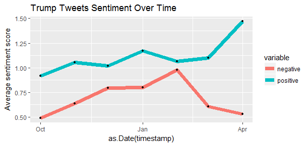
The positive sentiment scores are always higher than the negative sentiment scores. And the negative sentiment experienced a significant drop recently, the positive sentiment have increased to the highest point. However, the simple text mining process conducted in this post does not make this conclusion. A more sophisticated text analysis of Trump’s tweets by David Robinson found that Trump writes only the angrier half from Android, and another postive half from his staff using iPhone.
The end
I really enjoyed working on Trump Tweets analysis. Learning about text mining and social network analysis is very rewarding. Thanks to Julia Silge and Yanchang Zhao’s tutorials to make it possible.
Source code that created this post can be found here. I am happy to hear any feedback or questions.