
The H-1B program allows employers to temporarily employ foreign workers in the U.S on a nonimmigrant basis in specialty occupations. This is the most common visa status applied by international students after they complete higher education in the U.S and work in a full-time position. For those graduates to apply for H-1B visa, their employers must offer a job and petition for H-1B visa with the US immigration department.
The Office of Foreign Labor Certification (OFLC) generates program data. However, I downloaded the dataset from Kaggle directly after it has been mostly cleaned. To make it as relevant as possible, I will be only looking at the data from 2016.
I decide to remove all missing values, approximate 3% of applications were omitted. The data contains 629311 applications and 11 variables for 2016.
visa <- read.csv('h1b_kaggle.csv', stringsAsFactors = F)
visa <- visa[ which(visa$YEAR==2016),]
visa <- visa[complete.cases(visa[,-1]),]
str(visa)
##'data.frame': 629311 obs. of 11 variables:
## $ X : int 1 2 3 4 5 6 7 8 10 11 ...
## $ CASE_STATUS : chr "CERTIFIED-WITHDRAWN" "CERTIFIED-WITHDRAWN" ##"CERTIFIED-WITHDRAWN" "CERTIFIED-WITHDRAWN" ...
## $ EMPLOYER_NAME : chr "UNIVERSITY OF MICHIGAN" "GOODMAN NETWORKS, INC." ##"PORTS AMERICA GROUP, INC." "GATES CORPORATION, A WHOLLY-OWNED SUBSIDIARY OF ##TOMKINS PLC" ...
## $ SOC_NAME : chr "BIOCHEMISTS AND BIOPHYSICISTS" "CHIEF EXECUTIVES" ##"CHIEF EXECUTIVES" "CHIEF EXECUTIVES" ...
## $ JOB_TITLE : chr "POSTDOCTORAL RESEARCH FELLOW" "CHIEF OPERATING ##OFFICER" "CHIEF PROCESS OFFICER" "REGIONAL PRESIDEN, AMERICAS" ...
## $ FULL_TIME_POSITION: chr "N" "Y" "Y" "Y" ...
## $ PREVAILING_WAGE : num 36067 242674 193066 220314 157518 ...
## $ YEAR : int 2016 2016 2016 2016 2016 2016 2016 2016 2016 2016 ##...
## $ WORKSITE : chr "ANN ARBOR, MICHIGAN" "PLANO, TEXAS" "JERSEY CITY, ##NEW JERSEY" "DENVER, COLORADO" ...
## $ lon : num -83.7 -96.7 -74.1 -105 -90.2 ...
## $ lat : num 42.3 33 40.7 39.7 38.6 ...Throughout the analysis, I will attempt to answer the following questions:
- What are the top occupations America needs the most?
- Who are the top employers that submit the most applications?
- Which employers pay the most for what job?
- Which states and cities hire the most H-1B visa workers?
library(dplyr)
library(ggthemes)
library(ggplot2)
visa <- mutate_each(visa, funs(toupper))
visa$PREVAILING_WAGE <- as.numeric(visa$PREVAILING_WAGE)
visa$YEAR <- as.numeric(visa$YEAR)
visa$lon <- as.numeric(visa$lon)
visa$lat <- as.numeric(visa$lat)
occu_group <- group_by(visa, SOC_NAME)
visa_by_occu <- dplyr::summarize(occu_group,
                                 count = n(),
                                 mean = mean(PREVAILING_WAGE))
visa_by_occu <- visa_by_occu[with(visa_by_occu, order(-count)), ]
visa_by_occu <- visa_by_occu[1:20, ]
visa_by_occu$count[2] <- 114102
visa_by_occu= visa_by_occu[-6,]
What are the top occupations?
ggplot(aes(x = reorder(SOC_NAME, count), y=count), data = visa_by_occu) +
  geom_bar(stat = 'identity') + coord_flip() +
  xlab('Occupantions') +
  ylab('Number of Applications') +
  theme(axis.text = element_text(size = 8),
        plot.title = element_text(size = 12)) +
  ggtitle('Top H-1B Visa Occupations 2016')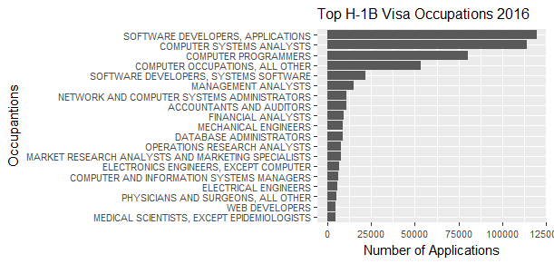
Technology related professions such as software developer, computer system analyst, programmer are among the most in demand occupations, analyst, accountant, engineer are among the second most in demand occupations.
Who are the top employers that submit the most applications?
employer_group <- group_by(visa, EMPLOYER_NAME)
visa_by_employer <- dplyr::summarize(employer_group,
                                     count = n(),
                                     mean = mean(PREVAILING_WAGE))
visa_by_employer <- visa_by_employer[with(visa_by_employer, order(-count)), ]
visa_by_employer <- visa_by_employer[1:20, ]
ggplot(aes(x = reorder(EMPLOYER_NAME, count), y=count), data = visa_by_employer) +
  geom_bar(stat = 'identity') + coord_flip() +
  xlab('Employers') +
  ylab('Number of Applications') +
  theme(axis.text = element_text(size = 7),
        plot.title = element_text(size = 10)) +
  ggtitle('Top Employers for H-1B Visa Application 2016')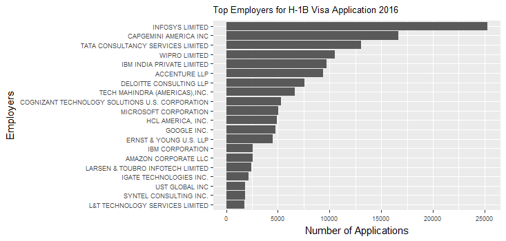
Infosys Limited leads by a large margin and submitted over 25000 applications last year. As a matter of fact, eight of the top 20 employers are Indian multinational IT companies.
employer_job_group <- group_by(visa, JOB_TITLE, EMPLOYER_NAME)
visa_by_employer_job <- dplyr::summarize(employer_job_group,
                                         count = n(),
                                         mean = mean(PREVAILING_WAGE))

visa_by_employer_job <- visa_by_employer_job[with(visa_by_employer_job, order(-count)), ]
visa_by_employer_job <- visa_by_employer_job[1:20, ]
ggplot(aes(x = reorder(JOB_TITLE, count), y=count, fill=EMPLOYER_NAME), data = visa_by_employer_job) +
  geom_bar(stat = 'identity', position = position_dodge()) +
  coord_flip() +
  ylab('Number of Applications') +
  xlab('Job Title') +
  theme(axis.text = element_text(size = 8),
        axis.text.x = element_text(angle = 90, hjust = 1, vjust = .4),
        legend.justification=c(1,0), legend.position=c(1,0), legend.title=element_text(size=8),
        legend.text=element_text(size=7),
        plot.title = element_text(size = 10)) +
  ggtitle('Top Job Titles for H-1B Visa Application 2016')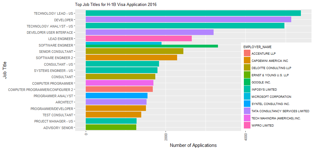
Technology leads and technology analysts are in huge demand at Infosys, developers and programmers are liked by Tata, Google is mainly interested in software engineers. Deloitte and Ernst & Young apply visa for consultants and advisors.
What occupations make the most Money?
When I look at prevailing wage distribution, I found something interesting.
summary(visa$PREVAILING_WAGE)##Min. 1st Qu. Median Mean 3rd Qu. Max.
## 0 57510 68410 89020 85180 329100000Minimum wage is 0 and maximum wage is 329100000. I suspected ‘0’s were missing values, and there are only five of them. But let’s have a look which company offered $329100000 and for what job.
visa[which.max(visa$PREVAILING_WAGE),]## X CASE_STATUS EMPLOYER_NAME SOC_NAME
##5275 5580 DENIED E AND D MEDIA INC. MARKETING MANAGERS
## JOB_TITLE FULL_TIME_POSITION PREVAILING_WAGE YEAR
##5275 DIRECTOR, SOCIAL AND DIGITAL MEDIA Y 329139200 2016
## WORKSITE lon lat
##5275 SANTA MONICA, CALIFORNIA -118.4912 34.01945For a digital media director? I am impressed. The application was denied anyway.
ggplot(aes(x = PREVAILING_WAGE), data = visa) +
  scale_x_continuous(limits = c(40000, 250000)) +
  geom_histogram(aes(y = ..density..),bins=50) + geom_density(color='blue') +
  xlab('Prevailing Wage(USD)') +
  ggtitle('Prevailing Wage Distribution 2016')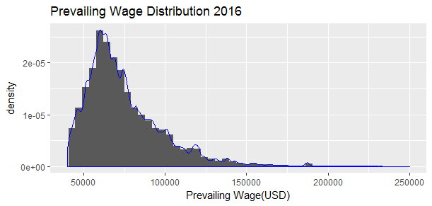
Majority of the prevailing wages were between 50K and 100K USD per annum.
ggplot(aes(x = reorder(SOC_NAME, mean), y=mean), data = visa_by_occu) +
  geom_bar(stat = 'identity') + coord_flip() +
  xlab('Occupantions') +
  ylab('Average Prevailing Wage(USD)') +
  theme(axis.text = element_text(size = 8),
        plot.title = element_text(size = 10)) +
ggtitle('Top Wage H-1B Visa Occupations 2016') 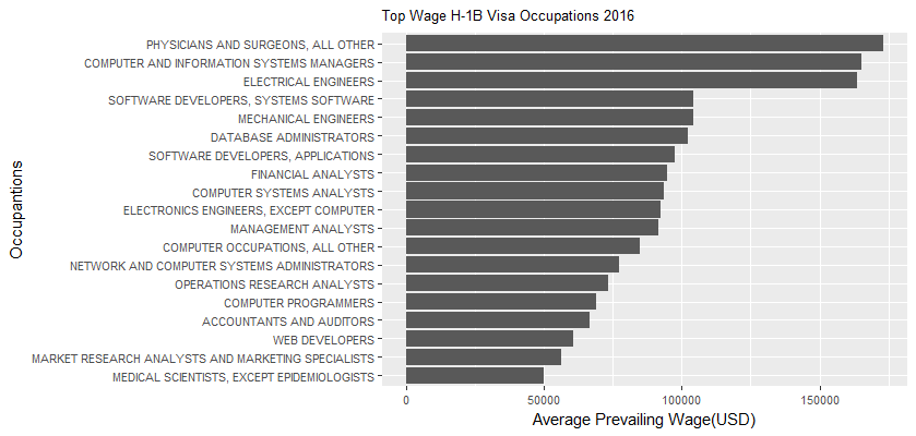
physicians and surgeons enjoy the highest average prevailing wages that almost reach $175K per annum last year, computer information systems managers and electrical engineers take the second spot make approximate $163K per annum last year.
Which Employers pay the most?
ggplot(aes(x = reorder(JOB_TITLE, mean), y=mean, fill=EMPLOYER_NAME), data = visa_by_employer_job) +
  geom_bar(stat = 'identity', position = position_dodge()) +
  coord_flip() +
  ylab('Average Prevailing Wage(USD)') +
  xlab('Job Title') +
  theme(axis.text = element_text(size = 8),
        axis.text.x = element_text(angle = 90, hjust = 1, vjust = .4),
        legend.justification=c(1,0), legend.position=c(1,0), legend.title=element_text(size=8), legend.text=element_text(size=7),
        plot.title = element_text(size = 9)) +
  ggtitle('Top Job Titles and Average Wages for H-1B Visa Application 2016')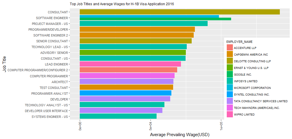
When comes to the job title and employer, consultants hired by Deloitte enjoy the highest average prevailing wage, software engineers hird by Google are paid far more than the same job title hired by the other companeis.
top_employer_df <- filter(visa, EMPLOYER_NAME %in% visa_by_employer[['EMPLOYER_NAME']])
ggplot(aes(x = EMPLOYER_NAME, y = PREVAILING_WAGE), data = top_employer_df) +
  geom_boxplot() +
  coord_flip(ylim=c(0,150000)) +
  xlab('Employers') +
  ylab('Prevailing Wage(USD)') +
  ggtitle('Wage by Top 20 Employers')
by(top_employer_df$PREVAILING_WAGE, top_employer_df$EMPLOYER_NAME, summary)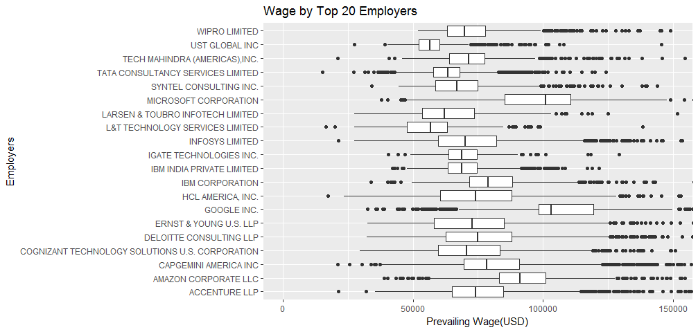
##top_employer_df$EMPLOYER_NAME: ACCENTURE LLP
##   Min. 1st Qu.  Median    Mean 3rd Qu.    Max.
##  21300   64940   74010   76420   84720  214900
##---------------------------------------------------------------
##top_employer_df$EMPLOYER_NAME: AMAZON CORPORATE LLC
##   Min. 1st Qu.  Median    Mean 3rd Qu.    Max.
##  39040   83140   91190   93590  101100  173100
##---------------------------------------------------------------
##top_employer_df$EMPLOYER_NAME: CAPGEMINI AMERICA INC
##   Min. 1st Qu.  Median    Mean 3rd Qu.    Max.
##  21050   69490   78400   81110   90790  229400
##---------------------------------------------------------------
##top_employer_df$EMPLOYER_NAME: COGNIZANT TECHNOLOGY SOLUTIONS U.S. CORPORATION
##   Min. 1st Qu.  Median    Mean 3rd Qu.    Max.
##  29560   59740   70550   72920   83390  163900
##---------------------------------------------------------------
##top_employer_df$EMPLOYER_NAME: DELOITTE CONSULTING LLP
##     Min.   1st Qu.    Median      Mean   3rd Qu.      Max.
##    32220     62750     74960     95000     87820 136800000
##---------------------------------------------------------------
##top_employer_df$EMPLOYER_NAME: ERNST & YOUNG U.S. LLP
##   Min. 1st Qu.  Median    Mean 3rd Qu.    Max.
##  32530   58180   72650   74120   85110  200900
##---------------------------------------------------------------
##top_employer_df$EMPLOYER_NAME: GOOGLE INC.
##   Min. 1st Qu.  Median    Mean 3rd Qu.    Max.
##  32550   98340  103100  105300  119400  221300
##---------------------------------------------------------------
##top_employer_df$EMPLOYER_NAME: HCL AMERICA, INC.
##   Min. 1st Qu.  Median    Mean 3rd Qu.    Max.
##  17260   60570   74090   75030   87840  165600
##---------------------------------------------------------------
##top_employer_df$EMPLOYER_NAME: IBM CORPORATION
##   Min. 1st Qu.  Median    Mean 3rd Qu.    Max.
##  33970   71580   78750   80920   88330  210400
##---------------------------------------------------------------
##top_employer_df$EMPLOYER_NAME: IBM INDIA PRIVATE LIMITED
##   Min. 1st Qu.  Median    Mean 3rd Qu.    Max.
##  42240   63320   68870   69880   74630 3277000
##---------------------------------------------------------------
##top_employer_df$EMPLOYER_NAME: IGATE TECHNOLOGIES INC.
##   Min. 1st Qu.  Median    Mean 3rd Qu.    Max.
##  40440   63690   68870   69720   74690  129300
##---------------------------------------------------------------
##top_employer_df$EMPLOYER_NAME: INFOSYS LIMITED
##   Min. 1st Qu.  Median    Mean 3rd Qu.    Max.
##  21300   59740   69970   72060   82200  180300
##---------------------------------------------------------------
##top_employer_df$EMPLOYER_NAME: L&T TECHNOLOGY SERVICES LIMITED
##   Min. 1st Qu.  Median    Mean 3rd Qu.    Max.
##  16600   47670   56760   56660   63170  138300
##---------------------------------------------------------------
##top_employer_df$EMPLOYER_NAME: LARSEN & TOUBRO INFOTECH LIMITED
##   Min. 1st Qu.  Median    Mean 3rd Qu.    Max.
##  27460   53520   62050   64040   73420  171400
##---------------------------------------------------------------
##top_employer_df$EMPLOYER_NAME: MICROSOFT CORPORATION
##   Min. 1st Qu.  Median    Mean 3rd Qu.    Max.
##  37750   85180  101100   99120  110600  173100
##---------------------------------------------------------------
##top_employer_df$EMPLOYER_NAME: SYNTEL CONSULTING INC.
##   Min. 1st Qu.  Median    Mean 3rd Qu.    Max.
##  34170   58680   66870   68780   74840  143700
##---------------------------------------------------------------
##top_employer_df$EMPLOYER_NAME: TATA CONSULTANCY SERVICES LIMITED
##     Min.   1st Qu.    Median      Mean   3rd Qu.      Max.
##    15220     57930     63460     73700     67890 133200000
##---------------------------------------------------------------
##top_employer_df$EMPLOYER_NAME: TECH MAHINDRA (AMERICAS),INC.
##     Min.   1st Qu.    Median      Mean   3rd Qu.      Max.
##    21200     64040     71430    189100     77600 170500000
##---------------------------------------------------------------
##top_employer_df$EMPLOYER_NAME: UST GLOBAL INC
##   Min. 1st Qu.  Median    Mean 3rd Qu.    Max.
##  27460   52190   56560   57500   60110  145400
##---------------------------------------------------------------
##top_employer_df$EMPLOYER_NAME: WIPRO LIMITED
##   Min. 1st Qu.  Median    Mean 3rd Qu.    Max.
##  51980   63150   69870   72750   77770  183900
Microsoft and Google offer the highest wages to their H-1B Visa workers. Their median wage exceeded $100K per annum, while the median wage of UST Global and L&T Technology are less than $60K per annum.
Which states and cities apply the most H-1B visas?
library(stringr)
visa$CITY <- str_replace(visa$WORKSITE, '(.+),.+', '\\1')
visa$STATE <- str_replace(visa$WORKSITE, '.+,(.+)', '\\1')
state_group <- group_by(visa, STATE)
visa_by_state <- dplyr::summarize(state_group,
                                  count = n(),
                                  mean = mean(PREVAILING_WAGE))
visa_by_state <- visa_by_state[with(visa_by_state, order(-count)), ]
visa_by_state <- visa_by_state[1:20, ]
ggplot(aes(x = reorder(STATE, count), y = count), data = visa_by_state) +
  geom_bar(stat = 'identity') + coord_flip() +
  xlab('State') +
  ylab('Number of Applications') +
  ggtitle('Top States Apply the Most H-1B Visas')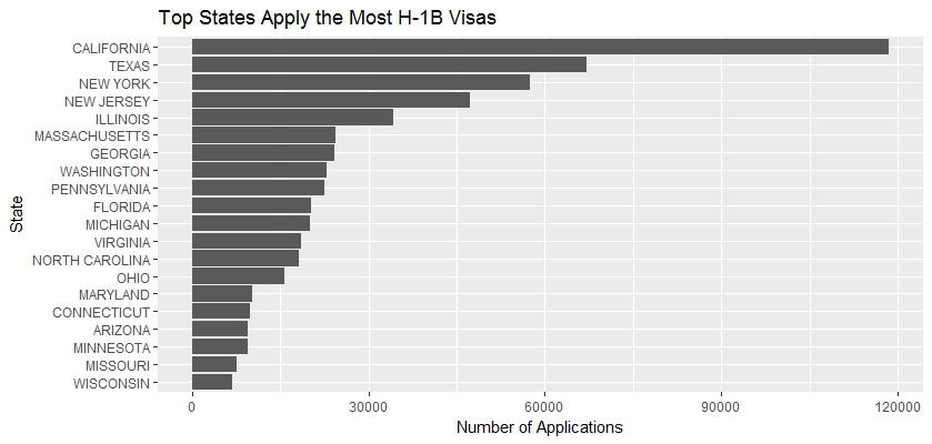
Expectedly, California hires the most workers on H-1B visas, followed by Texas, New York, New Jersey and Illinois.
city_group <- group_by(visa, CITY)
visa_by_city <- dplyr::summarize(city_group,
                                 count = n(),
                                 mean = mean(PREVAILING_WAGE))
visa_by_city <- visa_by_city[with(visa_by_city, order(-count)), ]
visa_by_city <- visa_by_city[1:20, ]
ggplot(aes(x = reorder(CITY, count), y = count), data = visa_by_city) +
  geom_bar(stat = 'identity') + coord_flip() +
  xlab('City') +
  ylab('Number of Applications') +
  ggtitle('Top Cities Apply the Most H-1B Visas')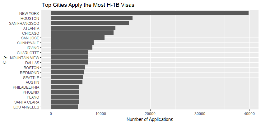
This time New York City takes the lead by a large margin in the number of H-1B Visa applications. Not only high tech companies in New York hire H-1B visa workers, but also New York’s fashion industry is heavily reliant on immigrants, from top designers to creative staffs to the sewing workers.
A Map of H-1B Visa Applications
states_map <- map_data("state")
ggplot(visa_state, aes(map_id = region)) +
    geom_map(aes(fill = count), map = states_map) +
    scale_colour_brewer(palette='Greens') +
    expand_limits(x = states_map$long, y = states_map$lat) +
  xlab('longitude') + ylab('latitude') + ggtitle('State H-1B Visa Applications')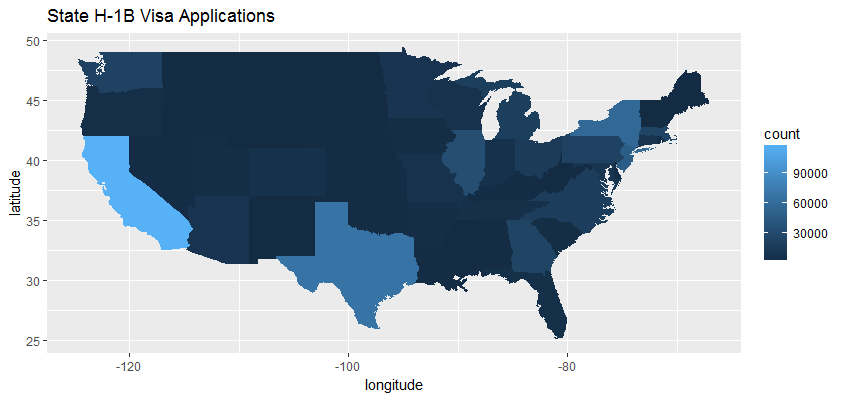
The End
It has been a great experience exploring 2016 H-1B visa petition data. With Trump’s Cracking down on the H-1B Visa program that Silicon Valley loves, I can’t wait to learn the data for 2017.
Source code that created this post can be found here. I am happy to hear any feedback or questions.