
I recently came across a R package called “unvote” that consists the voting history of countries in the United Nations General Assembly from 1946 to 2015. The packaged was developed by David Robinson.
Explore the data
library(ggplot2)
library(unvotes)
library(dplyr)
library(lubridate)
library(ggthemes)
library(tidyr)
The package contains three data set. The first is the history of each country’s vote, with more than 700,000 rows.
un_votes### A tibble: 738,764 × 4
## rcid country country_code vote
## <int> <chr> <chr> <fctr>
##1 3 United States of America US yes
##2 3 Canada CA no
##3 3 Cuba CU yes
##4 3 Haiti HT yes
##5 3 Dominican Republic DO yes
##6 3 Mexico MX yes
##7 3 Guatemala GT yes
##8 3 Honduras HN yes
##9 3 El Salvador SV yes
##10 3 Nicaragua NI yes
### ... with 738,754 more rowsThe second dataset contains information about each roll call vote, including the date, description, and relevant resolution that was voted on.
un_roll_calls### A tibble: 5,429 × 9
## rcid session importantvote date unres amend para
## <int> <dbl> <dbl> <date> <chr> <dbl> <dbl>
##1 3 1 0 1946-01-01 R/1/66 1 0
##2 4 1 0 1946-01-02 R/1/79 0 0
##3 5 1 0 1946-01-04 R/1/98 0 0
##4 6 1 0 1946-01-04 R/1/107 0 0
##5 7 1 0 1946-01-02 R/1/295 1 0
##6 8 1 0 1946-01-05 R/1/297 1 0
##7 9 1 0 1946-02-05 R/1/329 0 0
##8 10 1 0 1946-02-05 R/1/361 1 1
##9 11 1 0 1946-02-05 R/1/376 0 0
##10 12 1 0 1946-02-06 R/1/394 1 1
### ... with 5,419 more rows, and 2 more variables: short <chr>, descr <chr>The last data set contains relationships between each vote and six issues, they are “Palestinian conflict”, “Nuclear weapons and nuclear material”, “Arms control and disarmament”, “Human rights”, “Colonialism” and “Economic development”.
un_roll_call_issues### A tibble: 5,281 × 3
## rcid short_name issue
## <int> <chr> <chr>
##1 3372 me Palestinian conflict
##2 3658 me Palestinian conflict
##3 3692 me Palestinian conflict
##4 2901 me Palestinian conflict
##5 3020 me Palestinian conflict
##6 3217 me Palestinian conflict
##7 3298 me Palestinian conflict
##8 3429 me Palestinian conflict
##9 3558 me Palestinian conflict
##10 3625 me Palestinian conflict
### ... with 5,271 more rowsFirst, which issue(issues) have been voted the most?
un_roll_call_issues %>% count(issue, sort=TRUE)### A tibble: 6 × 2
## issue n
## <chr> <int>
##1 Palestinian conflict 1104
##2 Colonialism 991
##3 Human rights 986
##4 Arms control and disarmament 956
##5 Nuclear weapons and nuclear material 762
##6 Economic development 482How often a country voted “yes” from 1946 to 2015?
by_country <- un_votes %>% group_by(country) %>% summarize(votes = n(),
pct_yes = mean(vote == 'yes'))
by_country
### A tibble: 200 × 3
## country votes pct_yes
## <chr> <int> <dbl>
##1 Afghanistan 4972 0.8417136
##2 Albania 3514 0.7157086
##3 Algeria 4527 0.8981666
##4 Andorra 1564 0.6445013
##5 Angola 3075 0.9219512
##6 Antigua and Barbuda 2658 0.9194883
##7 Argentina 5361 0.7789591
##8 Armenia 1629 0.7587477
##9 Australia 5399 0.5523245
##10 Austria 4939 0.6329216
### ... with 190 more rowsPercentage yes vote high countries from 1946 to 2015
arrange(by_country, desc(pct_yes))### A tibble: 200 × 3
## country votes pct_yes
## <chr> <int> <dbl>
##1 Seychelles 1790 0.9782123
##2 Timor-Leste 837 0.9701314
##3 Sao Tome and Principe 2389 0.9673504
##4 Cabo Verde 3292 0.9599028
##5 Djibouti 3345 0.9563528
##6 Guinea Bissau 3070 0.9560261
##7 Comoros 2530 0.9450593
##8 Mozambique 3456 0.9427083
##9 United Arab Emirates 4031 0.9414537
##10 Suriname 3410 0.9410557
# ... with 190 more rowsPercentage yes vote low countries from 1946 to 2015
by_country[order(by_country$pct_yes),]### A tibble: 200 × 3
## country votes pct_yes
## <chr> <int> <dbl>
##1 Zanzibar 2 0.0000000
##2 United States of America 5390 0.2836735
##3 Palau 896 0.3225446
##4 Israel 4944 0.3460761
##5 Federal Republic of Germany 2067 0.3962264
##6 Micronesia (Federated States of) 1462 0.4138167
##7 United Kingdom of Great Britain and Northern Ireland 5372 0.4285182
##8 France 5325 0.4336150
##9 Marshall Islands 1600 0.4893750
##10 Belgium 5391 0.4952699
### ... with 190 more rowsPercentage yes vote high countries and years
join1 <- un_votes %>% inner_join(un_roll_calls, by = 'rcid')
by_country_year <- join1 %>% group_by(country, year=year(date)) %>% summarise(votes=n(), pct_yes = mean(vote=='yes'))
arrange(by_country_year, desc(pct_yes))
##Source: local data frame [9,689 x 4]
##Groups: country [200]
## country year votes pct_yes
## <chr> <dbl> <int> <dbl>
##1 Afghanistan 2002 40 1
##2 Afghanistan 2004 58 1
##3 Albania 1990 83 1
##4 Angola 1976 4 1
##5 Angola 1977 50 1
##6 Azerbaijan 2013 56 1
##7 Bahrain 1990 86 1
##8 Bahrain 1991 73 1
##9 Bahrain 1992 70 1
##10 Bahrain 1993 60 1
# ... with 9,679 more rowsPercentage yes vote low countries and years
by_country_year[order(by_country_year$pct_yes),]##Source: local data frame [9,689 x 4]
##Groups: country [200]
## country year votes pct_yes
## <chr> <dbl> <int> <dbl>
##1 Democratic Republic of the Congo 1998 1 0.00000000
##2 Jordan 1955 6 0.00000000
##3 Liberia 1998 1 0.00000000
##4 South Africa 1974 2 0.00000000
##5 Spain 1955 5 0.00000000
##6 Sri Lanka 1955 5 0.00000000
##7 Yugoslavia 1992 2 0.00000000
##8 Zanzibar 1963 2 0.00000000
##9 United States of America 1989 115 0.08695652
##10 United States of America 1988 134 0.09701493
### ... with 9,679 more rowsLet’s look at three countries - Canada, US and UK’s “Yes” vote trend in percent over year.
countries <- c('Canada', 'United States of America', 'United Kingdom of Great Britain and Northern Ireland')
by_country_year %>% filter(country %in% countries) %>%
  ggplot(aes(x=year, y=pct_yes, color=country)) + geom_line() +
  ylab("% of votes are 'Yes'") + ggtitle("Trend in percentage Yes Votes of Canada, US and UK 1946-2015") + theme_bw()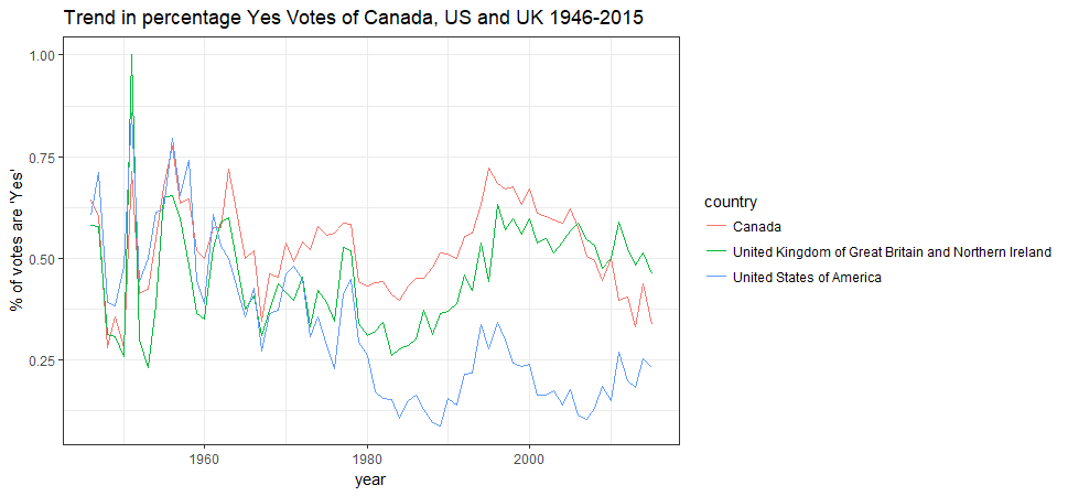
Let’s look at those six issues, how were they voted overtime by the above three countries?
join1 %>% filter(country %in% countries) %>%
  inner_join(un_roll_call_issues, by='rcid') %>%
  group_by(year=year(date), country, issue) %>%
  summarise(votes=n(), pct_yes=mean(vote=='yes')) %>%
  ggplot(aes(x=year, y=pct_yes, color=country)) +
  geom_point() +
  geom_smooth(se=FALSE) + facet_wrap(~issue) + ylab("% of votes are 'Yes'") +
  ggtitle('Trend in Percentage Yes Votes by Issues for Canada, US and UK')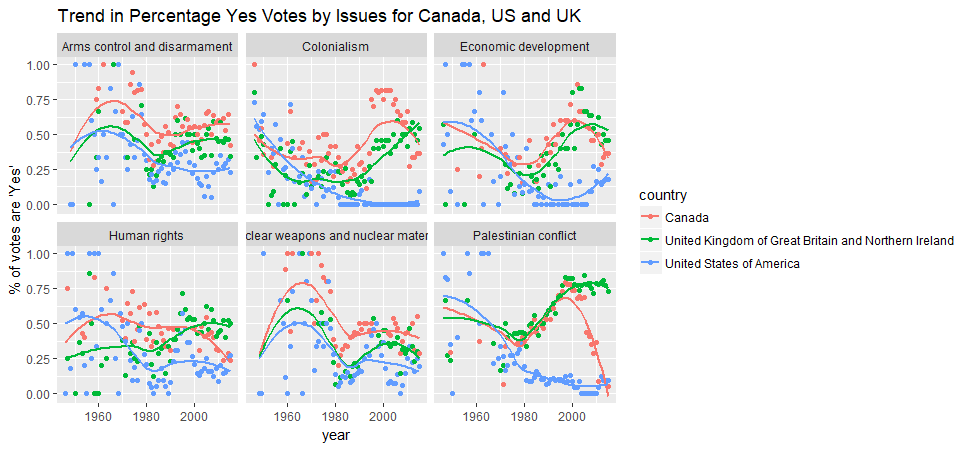
Among these three countries, which countries voted “yes” the most and the least for what issues?
join2 <- join1 %>% filter(country %in% countries) %>%
  inner_join(un_roll_call_issues, by='rcid') %>%
  group_by(country, issue) %>%
  summarise(votes=n(), pct_yes=mean(vote=='yes'))

ggplot(aes(x=country, y=pct_yes, fill = issue), data = join2) + geom_bar(stat = 'identity', position = position_dodge()) + ggtitle('Canada, US, UK and the UN Issues')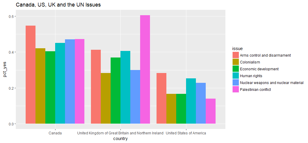
Let’s try to estimate the probability of these three countries’ changes in voting yes to the UN issues(i.e.whether there is a correlation between trend in year and percentage yes vote’)
us_by_year <- by_country_year %>% filter(country=='United States of America')
ca_by_year <- by_country_year %>% filter(country=='Canada')
uk_by_year <- by_country_year %>% filter(country=='United Kingdom of Great Britain and Northern Ireland')
us_model <- lm(pct_yes ~ year, data=us_by_year)
ca_model <- lm(pct_yes ~ year, data=ca_by_year)
uk_model <- lm(pct_yes ~ year, data = uk_by_year)
us_prob <- tidy(us_model) %>% filter(term=='year')
ca_prob <- tidy(ca_model) %>% filter(term=='year')
uk_prob <- tidy(uk_model) %>% filter(term=='year')
us_prob
ca_prob
uk_prob
##us_prob
## term estimate std.error statistic p.value
##1 year -0.007103352 0.0006991439 -10.16007 3.357004e-15
## ca_prob
## term estimate std.error statistic p.value
##1 year -0.0001975947 0.0006603795 -0.2992139 0.7657031
## uk_prob
## term estimate std.error statistic p.value
##1 year 0.00103754 0.0007739133 1.340641 0.184565Interpretation of the results
- For the USA, the probablity of voting yes to UN issues will decrease 0.0071 percent in the coming years; trend in year and percentage yes vote are highly correlated.
- For Canada, the probability of voting yes to UN issues will decrease 0.0002 percent in the coming years, and there is no correlation between trend in year and percentage yes vote.
- For the UK, the probability of voting yes to UN issues will decrease 0.001 percent in the coming years, and there is no correlation between trend in year and percentage yes vote.
The End
I realized that this package allows me to perform several statistical analysises including linear regression, logistic regression and I will save it to the next time.