
Load packages
library(ggplot2)
library(dplyr)
library(Hmisc)
library(corrplot)
Load data
load("brfss2013.RData")Part 1: About the Data
The Behavioral Risk Factor Surveillance System (BRFSS) is an annual telephone survey in the United States. The BRFSS is designed to identify risk factors in the adult population and report emerging trends. For example, respondents are asked about their diet and weekly physical activity, their HIV/AIDS status, possible tobacco use, immunization, health status, healthy days - health-related quality of life, health care access, inadequate sleep, hypertension awareness, cholesterol awareness, chronic health conditions, alcohol consumption, fruits and vegetables consumption, arthritis burden, and seatbelt use.
Data Collection:
Data collection procedure is explained in brfss_codebook. The data were collected from United States’ all 50 states, the District of Columbia, Puerto Rico, Guam and American Samoa, Federated States of Micronesia, and Palau, by conducting both landline telephone and cellular telephone-based surveys. Disproportionate stratified sampling (DSS) has been used for the landline sample and the cellular telephone respondents are randomly selected with each having equal probability of selection. The dataset we are working on contains 330 variables for a total of 491, 775 observations in 2013. The missing values denoted by “NA”.
Generalizability:
The sample data should allow us to generalize to the population of interest. It is a survey of 491,775 U.S. adults aged 18 years or older. It is based on a large stratified random sample. Potential biases are associated with non-response, incomplete interviews, missing values and convenience bias (some potential respondents may not have been included because they do not have a landline and cell phone).
Causality:
There is no causation can be established as BRFSS is an observation study that can only establish correlation/association between variables.
Part 2: Research Questions
Research quesion 1:
Does the distribution of the number of days in which physical and mental health was not good during the past 30 days differ by gender?
Research quesion 2:
Is there an association between the month in which a respondent was interviewed and the respondent’s self-reported health perception?
Research quesion 3:
Is there any association between income and health care coverage?
Research quesion 4:
Is there any relation between smoking, drinking alcohol, cholesterol level, blood pressure, weight and having a stroke? Eventually, I would like to see whether stroke can be predicted from the above mentioned variables.
Part 3: Exploratory data analysis
Research quesion 1:
ggplot(aes(x=physhlth, fill=sex), data = brfss2013[!is.na(brfss2013$sex), ]) +
  geom_histogram(bins=30, position = position_dodge()) + ggtitle('Number of Days Physical Health not Good in the Past 30 Days')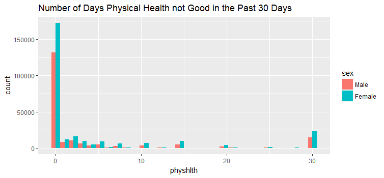
ggplot(aes(x=menthlth, fill=sex), data=brfss2013[!is.na(brfss2013$sex), ]) +
  geom_histogram(bins=30, position = position_dodge()) + ggtitle('Number of Days Mental Health not Good in the Past 30 Days')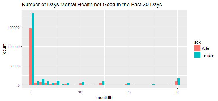
ggplot(aes(x=poorhlth, fill=sex), data=brfss2013[!is.na(brfss2013$sex), ]) +
  geom_histogram(bins=30, position = position_dodge()) + ggtitle('Number of Days with Poor Physical Or Mental Health in the Past 30 Days')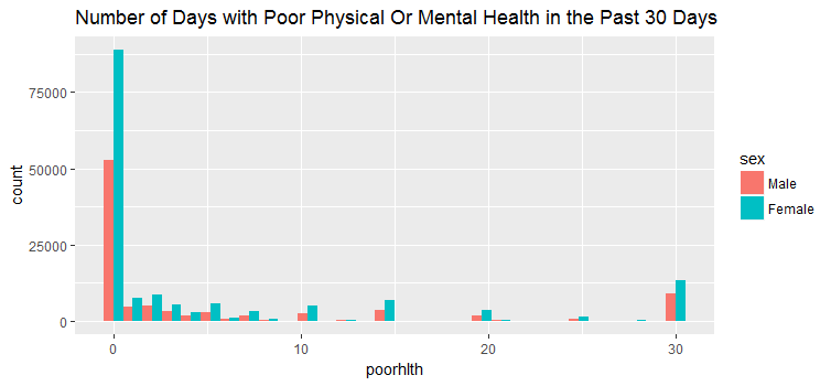
summary(brfss2013$sex)## Male Female NA's
##201313 290455 7 The above three figures show the data distribution of how male and female responded to the number of days physical, mental and both health not good during the past 30 days. We can see that there were far more female respondents than male respondents.
Research quesion 2:
by_month <- brfss2013 %>% filter(iyear=='2013') %>% group_by(imonth, genhlth) %>% summarise(n=n())
ggplot(aes(x=imonth, y=n, fill = genhlth), data = by_month[!is.na(by_month$genhlth), ]) + geom_bar(stat = 'identity', position = position_dodge()) + ggtitle('Health Perception By Month')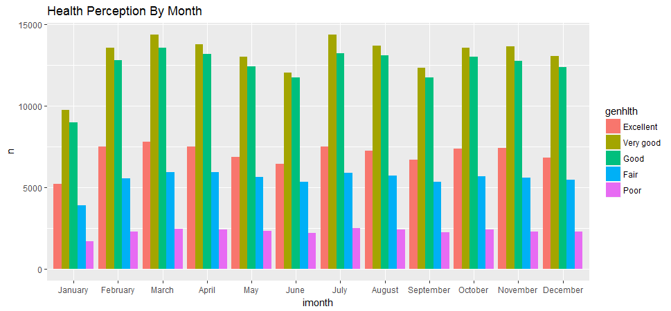
by_month1 <- brfss2013 %>% filter(iyear=='2013') %>% group_by(imonth) %>% summarise(n=n())
ggplot(aes(x=imonth, y=n), data=by_month1) + geom_bar(stat = 'identity') + ggtitle('Number of Respondents by Month')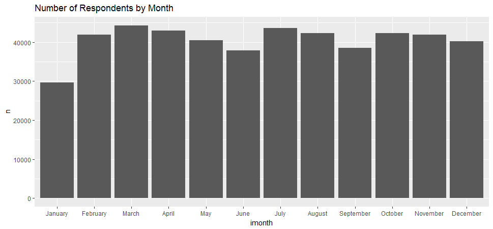
I was trying to find out whether people respond their health condition differently in the different month. For example, are people more likely to say they are in good health in the spring or summer? It appears that there was no obvious pattern.
Research quesion 3:
plot(brfss2013$income2, brfss2013$hlthpln1, xlab = 'Income Level', ylab = 'Health Care Coverage', main =
'Income Level versus Health Care Coverage')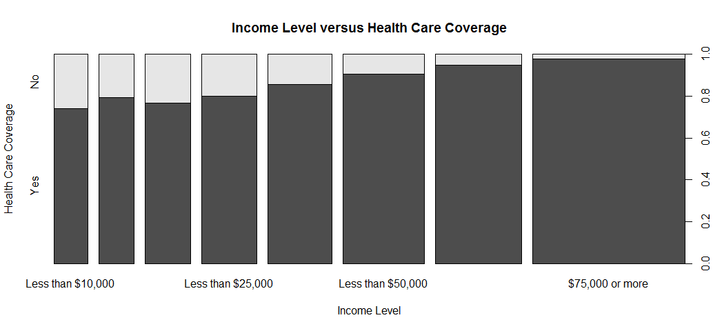
In general, higher income respondents are more likely to have health care coverage then those of lower income respondents.
Research quesion 4:
To answer this question, I willl be using the following varibles:
-
smoke100: Smoked At Least 100 Cigarettes
-
avedrnk2: Avg Alcoholic Drinks Per Day In Past 30
-
bphigh4: Ever Told Blood Pressure High
-
toldhi2: Ever Told Blood Cholesterol High
-
weight2: Reported Weight In Pounds
-
cvdstrk3: Ever Diagnosed With A Stroke
First, convert the above variables to numeric, and see any correlation between these numerica variables.
vars <- names(brfss2013) %in% c('smoke100', 'avedrnk2', 'bphigh4', 'toldhi2', 'weight2')
selected_brfss <- brfss2013[vars]
selected_brfss$toldhi2 <- ifelse(selected_brfss$toldhi2=="Yes", 1, 0)
selected_brfss$smoke100 <- ifelse(selected_brfss$smoke100=="Yes", 1, 0)
selected_brfss$weight2 <- as.numeric(selected_brfss$weight2)
selected_brfss$bphigh4 <- as.factor(ifelse(selected_brfss$bphigh4=="Yes", "Yes", (ifelse(selected_brfss$bphigh4=="Yes, but female told only during pregnancy", "Yes", (ifelse(selected_brfss$bphigh4=="Told borderline or pre-hypertensive", "Yes", "No"))))))
selected_brfss$bphigh4 <- ifelse(selected_brfss$bphigh4=="Yes", 1, 0)
selected_brfss <- na.delete(selected_brfss)
corr.matrix <- cor(selected_brfss)
corrplot(corr.matrix, main="\n\nCorrelation Plot of Smoke, Alcohol, Blood pressure, Cholesterol, and Weight", method="number")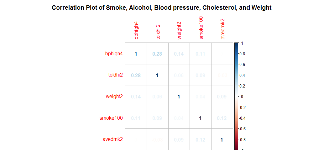
No any two numeric variables seem to have strong correlations.
Logistic Regression to Predict Stroke
Replace the answer “Yes, but female told only during pregnancy” and “Told borderline or pre-hypertensive” with “Yes”.
vars1 <- names(brfss2013) %in% c('smoke100', 'avedrnk2', 'bphigh4', 'toldhi2', 'weight2', 'cvdstrk3')
stroke <- brfss2013[vars1]
stroke$bphigh4 <- as.factor(ifelse(stroke$bphigh4=="Yes", "Yes", (ifelse(stroke$bphigh4=="Yes, but female told only during pregnancy", "Yes", (ifelse(stroke$bphigh4=="Told borderline or pre-hypertensive", "Yes", "No"))))))
stroke$weight2<-as.numeric(stroke$weight2)
Replace ‘NA’ values with ‘No’.
stroke$bphigh4 <- replace(stroke$bphigh4, which(is.na(stroke$bphigh4)), "No")
stroke$toldhi2 <- replace(stroke$toldhi2, which(is.na(stroke$toldhi2)), "No")
stroke$cvdstrk3 <- replace(stroke$cvdstrk3, which(is.na(stroke$cvdstrk3)), "No")
stroke$smoke100 <- replace(stroke$smoke100, which(is.na(stroke$smoke100)), 'No')
Replace ‘NA’ value by average.
mean(stroke$avedrnk2,na.rm = T)##[1] 2.209905stroke$avedrnk2 <- replace(stroke$avedrnk2, which(is.na(stroke$avedrnk2)), 2)Have a look the data that will be used for modeling.
head(stroke)
summary(stroke)
## bphigh4 toldhi2 cvdstrk3 weight2 smoke100 avedrnk2
##1 Yes Yes No 154 Yes 2
##2 No No No 30 No 2
##3 No No No 63 Yes 4
##4 No Yes No 31 No 2
##5 Yes No No 169 Yes 2
##6 Yes Yes No 128 No 2## bphigh4 toldhi2 cvdstrk3 weight2 smoke100
## No :284107 Yes:183501 Yes: 20391 Min. : 1.00 Yes:215201
## Yes:207668 No :308274 No :471384 1st Qu.: 43.00 No :276574
## Median : 73.00
## Mean : 80.22
## 3rd Qu.:103.00
## Max. :570.00
## avedrnk2
## Min. : 1.000
## 1st Qu.: 2.000
## Median : 2.000
## Mean : 2.099
## 3rd Qu.: 2.000
## Max. :76.000 Covert to binary outcome.
stroke$cvdstrk3 <- ifelse(stroke$cvdstrk3=="Yes", 1, 0)After wrangling and cleaning the data, now we can fit the model.
Logistic Regression Model Fitting
train <- stroke[1:390000,]
test <- stroke[390001:491775,]
model <- glm(cvdstrk3 ~.,family=binomial(link = 'logit'),data=train)
summary(model)
##Call:
##glm(formula = cvdstrk3 ~ ., family = binomial(link = "logit"),
## data = train)
##Deviance Residuals:
## Min 1Q Median 3Q Max
##-0.5057 -0.3672 -0.2109 -0.1630 3.2363
##Coefficients:
## Estimate Std. Error z value Pr(>|z|)
##(Intercept) -3.2690106 0.0268240 -121.869 < 2e-16 ***
##bphigh4Yes 1.3051850 0.0193447 67.470 < 2e-16 ***
##toldhi2No -0.5678048 0.0171500 -33.108 < 2e-16 ***
##weight2 -0.0009628 0.0001487 -6.476 9.41e-11 ***
##smoke100No -0.3990598 0.0163896 -24.348 < 2e-16 ***
##avedrnk2 -0.0274511 0.0065099 -4.217 2.48e-05 ***
##---
##Signif. codes: 0 '***' 0.001 '**' 0.01 '*' 0.05 '.' 0.1 ' ' 1
##(Dispersion parameter for binomial family taken to be 1)
## Null deviance: 136364 on 389999 degrees of freedom
##Residual deviance: 126648 on 389994 degrees of freedom
##AIC: 126660
##Number of Fisher Scoring iterations: 6Interpreting the results of my logistic regression model:
All the variables are statistically significant.
-
All other variables being equal, being told blood pressure high is more likely to have a stroke.
-
The negative coefficient for the predictor - toldhi2No suggests that all other variables being equal, not being told blood cholesterol high is less likely to have a stroke.
-
For every one unit change in weight, the log odds of having a stroke (versus no-stroke) decreases by 0.00096.
-
Not Smoked At Least 100 Cigarettes, less likely to have a stroke.
-
For a one unit increase in Avg alcoholic drinks per day in past 30 days, the log odds of having a stroke decreases by 0.027.
anova(model, test="Chisq")##Analysis of Deviance Table
##Model: binomial, link: logit
##Response: cvdstrk3
##Terms added sequentially (first to last)
## Df Deviance Resid. Df Resid. Dev Pr(>Chi)
##NULL 389999 136364
##bphigh4 1 7848.6 389998 128516 < 2.2e-16 ***
##toldhi2 1 1230.1 389997 127285 < 2.2e-16 ***
##weight2 1 33.2 389996 127252 8.453e-09 ***
##smoke100 1 584.5 389995 126668 < 2.2e-16 ***
##avedrnk2 1 19.9 389994 126648 7.958e-06 ***
##---
##Signif. codes: 0 '***' 0.001 '**' 0.01 '*' 0.05 '.' 0.1 ' ' 1Analyzing the deviance table we can see the drop in deviance when adding each variable one at a time. Adding bphigh4, toldhi2, smoke100 significantly reduces the residual deviance. The other variables weight2 and avedrnk2 seem to imrove the model less even though they all have low p-values.
Assessing the predictive ability of the model
fitted.results <- predict(model,newdata=test,type='response')
fitted.results <- ifelse(fitted.results > 0.5,1,0)

misClasificError <- mean(fitted.results != test$cvdstrk3)
print(paste('Accuracy',1-misClasificError))
##[1] "Accuracy 0.961296978629329The 0.96 accuracy on the test set is a very good result.
Plot the ROC curve and calculate the AUC (area under the curve).
library(ROCR)
p <- predict(model, newdata=test, type="response")
pr <- prediction(p, test$cvdstrk3)
prf <- performance(pr, measure = "tpr", x.measure = "fpr")
plot(prf)
auc <- performance(pr, measure = "auc")
auc <- auc@y.values[[1]]
auc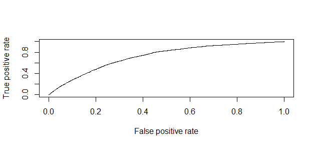
##[1] 0.7226642One last note, when we analyze health survery data, we must be aware that self-reported prevalence may be biased because respondents may not be aware of their risk status. Therefore, to achieve more precise estimates, researchers are using laboratory tests as well as self-reported data.
Source code that created this post can be found here. I am happy to hear any feedback and questions.