
Warren Buffett released the most recent version of his annual letter to Berkshire Hathaway shareholders a couple of months ago. After reading a post regarding a sentiment analysis of Mr Warren Buffett’s annual shareholder letters, and I am also learning text mining with R. I thought it is a great opportunity to apply my latest skills into practice, - text mining 40 years of Warren Buffett’s letters to shareholders.
library(dplyr)
library(ggplot2)
library(tidyr)
library(tidytext)
library(pdftools)
library(rvest)
library(XML)
library(stringr)
library(ggthemes)
The code I used here to download all the letters were borrowed from Michael Toth.
urls_77_97 <- paste('http://www.berkshirehathaway.com/letters/', seq(1977, 1997), '.html', sep='')
html_urls <- c(urls_77_97,
               'http://www.berkshirehathaway.com/letters/1998htm.html',
               'http://www.berkshirehathaway.com/letters/1999htm.html',
               'http://www.berkshirehathaway.com/2000ar/2000letter.html',
               'http://www.berkshirehathaway.com/2001ar/2001letter.html')

letters_html <- lapply(html_urls, function(x) read_html(x) %>% html_text())

# Getting & Reading in PDF Letters
urls_03_16 <- paste('http://www.berkshirehathaway.com/letters/', seq(2003, 2016), 'ltr.pdf', sep = '')
pdf_urls <- data.frame('year' = seq(2002, 2016),
                       'link' = c('http://www.berkshirehathaway.com/letters/2002pdf.pdf', urls_03_16))

download_pdfs <- function(x) {
  myfile = paste0(x['year'], '.pdf')
  download.file(url = x['link'], destfile = myfile, mode = 'wb')
  return(myfile)
}

pdfs <- apply(pdf_urls, 1, download_pdfs)
letters_pdf <- lapply(pdfs, function(x) pdf_text(x) %>% paste(collapse=" "))
tmp <- lapply(pdfs, function(x) if(file.exists(x)) file.remove(x)) # Clean up directory

# Combine all letters in a data frame
letters <- do.call(rbind, Map(data.frame, year=seq(1977, 2016), text=c(letters_html, letters_pdf)))
letters$text <- as.character(letters$text)
Now I am ready to use “unnest_tokens” to split the dataset(all the letters) into tokens and remove stop words.
letter_words <- letters %>%
  unnest_tokens(word, text) %>%
  filter(str_detect(word, "[a-z']$"),
         !word %in% stop_words$word)
The most common words throughout 40 years of letters
letter_words %>%
  count(word, sort=TRUE)
### A tibble: 14,788 × 2
## word n
## <chr> <int>
##1 business 2143
##2 berkshire 1992
##3 earnings 1863
##4 company 1241
##5 million 1224
##6 insurance 1171
##7 businesses 982
##8 companies 823
##9 market 771
##10 billion 760
### ... with 14,778 more rowsletter_words %>%
count(word, sort = TRUE) %>%
filter(n > 600) %>%
mutate(word = reorder(word, n)) %>%
ggplot(aes(word, n)) +
geom_col() +
xlab(NULL) +
coord_flip() + ggtitle("The Most Common Words in Buffett's Letters") + theme_minimal()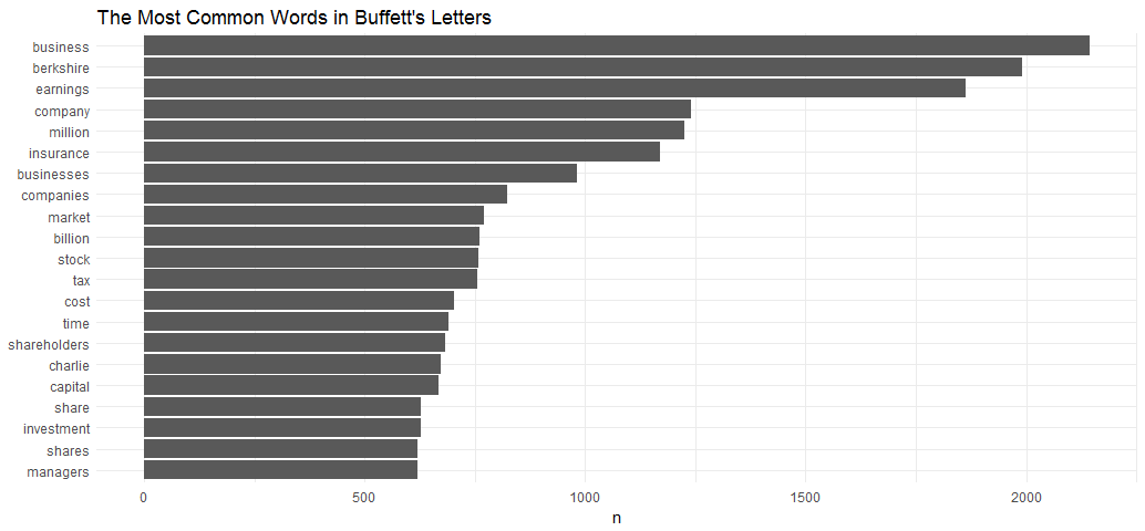
The most common words each year
words_by_year <- letter_words %>%
  count(year, word, sort = TRUE) %>%
  ungroup()
words_by_year
### A tibble: 83,537 × 3
## year word n
## <int> <chr> <int>
##1 2014 berkshire 203
##2 1985 business 112
##3 1983 business 97
##4 1984 business 96
##5 2014 business 92
##6 1990 business 90
##7 2015 berkshire 90
##8 1980 earnings 87
##9 2016 berkshire 86
##10 1989 business 85
### ... with 83,527 more rowsSentiment by Year
Examine how often positive and negative words occurred in these letters. Which years were the most positive or negative overall?
AFINN lexion provides a positivity score for each word, from -5 (most negative) to 5 (most positive). What I am doing here is to calculate the average sentiment score for each year.
letters_sentiments <- words_by_year %>%
  inner_join(get_sentiments("afinn"), by = "word") %>%
  group_by(year) %>%
  summarize(score = sum(score * n) / sum(n))

letters_sentiments %>%
  mutate(year = reorder(year, score)) %>%
  ggplot(aes(year, score, fill = score > 0)) +
  geom_col(show.legend = FALSE) +
  coord_flip() +
  ylab("Average sentiment score") +
  ggtitle("Sentiment Score of Buffett's Letters to Shareholders 1977-2016") + theme_minimal()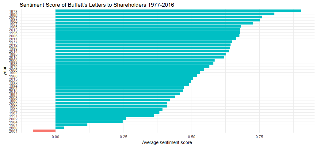
Warren Buffett is known for his long-term, optimistic economic outlook. Only 1 out of 40 letters appeared negative. Berkshire’s loss in net worth during 2001 was $3.77 billion, in addition, 911 terrorist attack contributed to the negative sentiment score in that year’s letter.
Sentiment Analysis by Words
Examine the total positive and negative contributions of each word.
contributions <- letter_words %>%
  inner_join(get_sentiments("afinn"), by = "word") %>%
  group_by(word) %>%
  summarize(occurences = n(),
            contribution = sum(score))
contributions
### A tibble: 1,225 × 3
## word occurences contribution
## <chr> <int> <int>
##1 abandon 4 -8
##2 abandoned 4 -8
##3 abhor 2 -6
##4 abilities 12 24
##5 ability 96 192
##6 aboard 3 3
##7 absentee 6 -6
##8 absorbed 3 3
##9 abuse 2 -6
##10 abuses 1 -3
### ... with 1,215 more rowsFor example, word “abandon” appeared 4 times and contributed total -8 scores.
contributions %>%
  top_n(25, abs(contribution)) %>%
  mutate(word = reorder(word, contribution)) %>%
  ggplot(aes(word, contribution, fill = contribution > 0)) +
  geom_col(show.legend = FALSE) +
  coord_flip() + ggtitle('Words with the Most Contributions to Positive/Negative Sentiment Scores') + theme_minimal()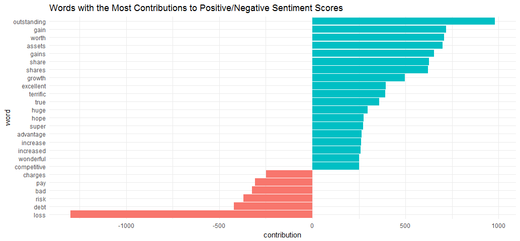
Word “outstanding” made the most positive contribution and word “loss” made the most negative contribution.
sentiment_messages <- letter_words %>%
  inner_join(get_sentiments("afinn"), by = "word") %>%
  group_by(year, word) %>%
  summarize(sentiment = mean(score),
            words = n()) %>%
  ungroup() %>%
  filter(words >= 5)
sentiment_messages %>%
  arrange(desc(sentiment))
### A tibble: 763 × 4
## year word sentiment words
## <int> <chr> <dbl> <int>
##1 1979 outstanding 5 6
##2 1984 outstanding 5 7
##3 1986 outstanding 5 7
##4 1988 superb 5 5
##5 1989 outstanding 5 5
##6 1989 superb 5 6
##7 1992 outstanding 5 7
##8 1995 outstanding 5 9
##9 1996 outstanding 5 9
##10 1997 outstanding 5 5Now we look for the words with the highest positive scores in each letter, here it is, “outstanding” appeared eight out of ten letters.
sentiment_messages %>%
  arrange(sentiment)
### A tibble: 763 × 4
## year word sentiment words
## <int> <chr> <dbl> <int>
##1 1979 loss -3 5
##2 1980 loss -3 6
##3 1981 bad -3 7
##4 1982 loss -3 6
##5 1983 loss -3 8
##6 1984 bad -3 5
##7 1984 charged -3 6
##8 1984 loss -3 23
##9 1985 loss -3 18
##10 1986 loss -3 15
### ... with 753 more rowsUnsurprisingly, seven out of ten letters, word “loss” secured the highest negative score.
From doing text mining Google finance articles a few days ago, I have learned another sentiment lexicon - “loughran”, which was developed based on analyses of financial reports. The Loughran dictionary divides words into six sentiments: “positive”, “negative”, “litigious”, “uncertainty”, “constraining”, and “superfluous”. I can’t wait to apply this dictionary to Buffett’s letters.
letter_words %>%
  count(word) %>%
  inner_join(get_sentiments("loughran"), by = "word") %>%
  group_by(sentiment) %>%
  top_n(5, n) %>%
  ungroup() %>%
  mutate(word = reorder(word, n)) %>%
  ggplot(aes(word, n)) +
  geom_col() +
  coord_flip() +
  facet_wrap(~ sentiment, scales = "free") +
  ggtitle("Frequency of This Word in Buffett's Letters") + theme_minimal()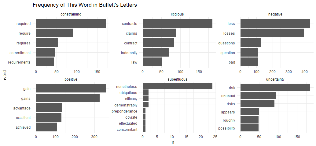
The assignments of words to sentments look reasonable. However, it removed “outstanding” and “superb” from the positive sentiment.
Relationship Between Words
Now it is the most interesting part. By tokenizing text into consecutive sequences of words, we can examine how often one word is followed by another. We can then study the relationship between words.
In this case, defining a list of six words that are used in negative situation, such as “don’t”, “not”, “no”, “can’t”, “won’t” and “without”, and visualize the sentiment-associated words that most often followed them.
letters_bigrams <- letters %>%
  unnest_tokens(bigram, text, token = "ngrams", n = 2)
letters_bigram_counts <- letters_bigrams %>%
  count(year, bigram, sort = TRUE) %>%
  ungroup() %>%
  separate(bigram, c("word1", "word2"), sep = " ")

negate_words <- c("not", "without", "no", "can't", "don't", "won't")

letters_bigram_counts %>%
  filter(word1 %in% negate_words) %>%
  count(word1, word2, wt = n, sort = TRUE) %>%
  inner_join(get_sentiments("afinn"), by = c(word2 = "word")) %>%
  mutate(contribution = score * nn) %>%
  group_by(word1) %>%
  top_n(10, abs(contribution)) %>%
  ungroup() %>%
  mutate(word2 = reorder(paste(word2, word1, sep = "__"), contribution)) %>%
  ggplot(aes(word2, contribution, fill = contribution > 0)) +
  geom_col(show.legend = FALSE) +
  facet_wrap(~ word1, scales = "free", nrow = 3) +
  scale_x_discrete(labels = function(x) gsub("__.+$", "", x)) +
  xlab("Words followed by a negation") +
  ylab("Sentiment score * # of occurrences") +
  theme(axis.text.x = element_text(angle = 90, hjust = 1)) +
  coord_flip() + ggtitle("Words that contributed the most to sentiment when they followed a ‘negation'") + theme_minimal()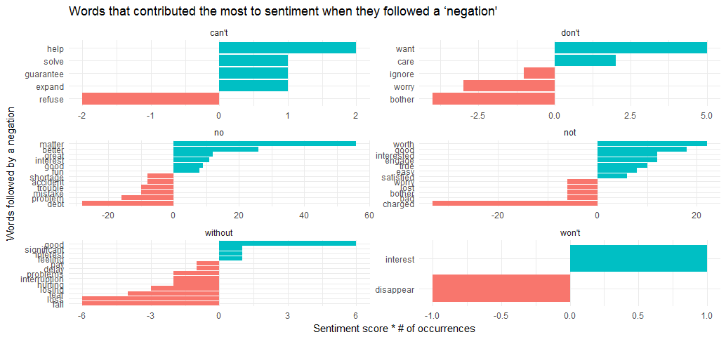
It looks like the largest sources of misidentifying a word as positive come from “no matter”, “no better”, “not worth”, “not good”, and the largest source of incorrectly classified negative sentiment is “no debt”, “no problem” and “not charged”.
Source code that created this post can be found here. I am happy to hear any feedback or questions.
Reference: